pointcoral

pointcoral is a local, open-source R package for CPCe/photoquadrat point-count workflows. It imports CPCe point annotations, matches those points to source images, creates ecological percent-cover tables, writes visual QC overlays, and exports machine-learning-ready point labels, image-centered patches, sparse masks, and train/validation/test splits. When you want richer labels, it can also standardize raw short labels with a flexible crosswalk.

The package is designed for reef photoquadrat projects where the raw CPCe labels are project-specific shorthand codes such as SPO, CALG, PEYS, LOBO, or S. Those raw labels are already inside the .cpc files and are always preserved. You can run a bare workflow directly from those labels. A crosswalk is the optional bonus layer that maps them to full species or benthic type labels such as Sponge, Coralline algae, Peyssonnelia, Lobophora variegata, or Sand, plus the ecological major classes and subclasses used for analysis.

pointcoral does not depend on MERMAID, mermaidr, CoralNet accounts, cloud APIs, Python, or any closed platform. It is built to run fully on your own computer with your own files.

Reference

The CPCe software and random point-count method are described in:

Kohler, K.E. and S.M. Gill (2006). “Coral Point Count with Excel extensions (CPCe): A Visual Basic program for the determination of coral and substrate coverage using random point count methodology.” Computers & Geosciences 32(9): 1259-1269. DOI: 10.1016/j.cageo.2005.11.009.

What this looks like

The package starts with CPCe files and reef images, then produces clean tables, summary graphics, QC images, and ML-ready outputs. The examples below are built from the two bundled sample .cpc files and matching sample images included in this repository.

1. Optional standardization turns raw CPCe labels into readable labels

CPCe stores short codes. pointcoral keeps those short codes but joins them to the full label and ecological class you define in a crosswalk when you provide one.

2. Imported points become a tidy table

Each CPCe point is converted into a row with image identity, pixel coordinates, and the original raw label. After the optional crosswalk step, the same table also includes full labels, ecological classes, and class IDs.

3. Percent-cover summaries are created automatically

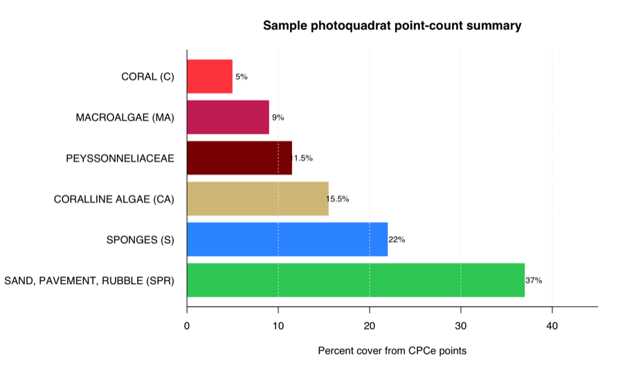
This figure summarizes the two bundled sample images after applying the bundled example crosswalk. The numbers are still computed directly from CPCe point counts. Without a crosswalk, the same summary functions report percent cover by raw_label.

The same results are also written as CSV tables. For example, image-level output looks like this:

4. QC overlays show whether points landed in the right place

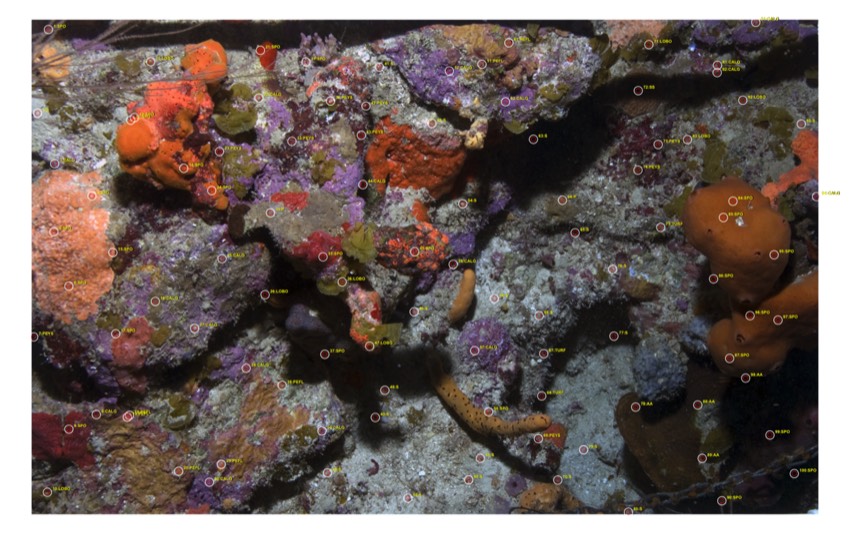
The package writes annotated images so you can inspect CPCe point placement and labels before trusting summaries or ML exports.

5. ML patch datasets can be made from the same points

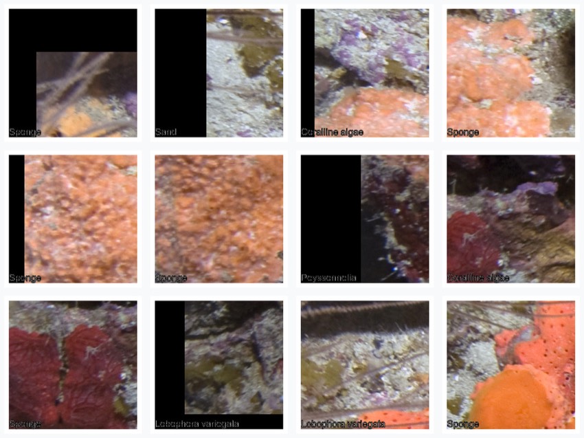
Each point can become an image-centered crop. These patches can be used for patch classification, active learning, review workflows, or as weak labels for model development.

6. Sparse masks are weak segmentation labels

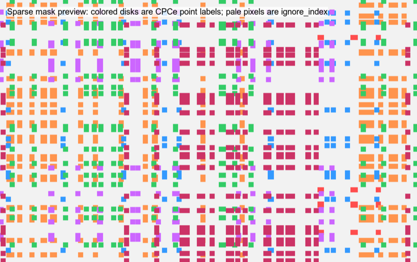
Sparse masks only label a small disk around each CPCe point. The pale background is ignore_index, meaning it is not treated as a dense annotation.

7. Potential ML outputs from pointcoral data

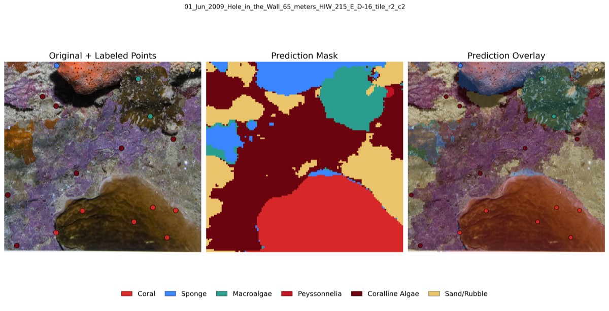
Pointcoral point tables can support downstream ML review products such as labeled point views, prediction masks, and prediction overlays.

Installation

Install from GitHub:

install.packages("remotes")
remotes::install_github("el-cordero/pointcoral")

Load the package:

library(pointcoral)

What pointcoral expects

At minimum you need:

1. CPCe .cpc files or CPCe-like point export tables.
2. Matching image files.

A simple project folder can look like this:

my_project/
  cpce/
    HIW_158_W_U-1.cpc
    H_211_E_U-1.cpc
  images/
    HIW_158_W_U-1.jpg
    H_211_E_U-1.jpg
  outputs/

The .cpc files and images may also live in the same folder. Image matching is by basename, so HIW_158_W_U-1.cpc matches HIW_158_W_U-1.jpg.

A crosswalk is optional. Add one when you want to translate raw CPCe labels into full labels, major ecological classes, subclasses, or project-specific ML classes:

my_project/
  labels/
    my_crosswalk.csv

Important label model

The package uses this distinction:

• raw_code: the original CPCe short code.
• raw_label: also the original CPCe short code as it appeared in the .cpc.
• full_label: the full species or benthic type name. This usually comes from a crosswalk, not from the bare .cpc point rows.
• clean_label: the standardized analysis label. By default this is the same as full_label.
• label_class: an optional subclass/type field, such as subcategory, artifact, or disease_or_condition.
• major_category: the ecological major class, such as CORAL (C), SPONGES (S), PEYSSONNELIACEAE, or SAND, PAVEMENT, RUBBLE (SPR).
• ml_class: the class label used for ML exports after standardization. In a bare workflow, pointcoral uses raw_label instead.
• class_id: integer ID for ML masks and class lookup tables. If a crosswalk does not provide IDs, IDs are generated from the label column being used.

For example:

raw_code raw_label full_label                label_class major_category
SPO      SPO       Sponge                    subcategory SPONGES (S)
CALG     CALG      Coralline algae           subcategory CORALLINE ALGAE (CA)
PEFL     PEFL      Peyssonnelia flavescens   subcategory PEYSSONNELIACEAE
LOBO     LOBO      Lobophora variegata       subcategory MACROALGAE (MA)
S        S         Sand                      subcategory SAND, PAVEMENT, RUBBLE (SPR)

The bundled example crosswalk is a starting example, not a universal ontology. You do not need it for the bare workflow, but you should review it against your own CPCe codefile before using standardized classes for final analysis.

Quick start with bundled example data

The package includes two small .cpc files and matching JPEGs in inst/extdata.

library(pointcoral)
library(dplyr)

example_dir <- system.file("extdata", package = "pointcoral")

points_raw <- read_cpce_folder(
  path = example_dir,
  image_root = example_dir,
  recursive = FALSE
)

points_raw |>
  select(image_id, point_id, x_px, y_px, raw_label) |>
  head()

Bare example output:

image_id       point_id x_px y_px raw_label
HIW_158_W_U-1 1        65   38    SPO
HIW_158_W_U-1 2        23   362   S
HIW_158_W_U-1 3        89   557   CALG

You can summarize immediately by raw CPCe label:

summarize_images(points_raw)

Then, as an optional standardization step, add the example crosswalk:

crosswalk_path <- system.file(
  "extdata",
  "pointcoral_example_crosswalk.csv",
  package = "pointcoral"
)

crosswalk <- read_label_crosswalk(crosswalk_path)
points_clean <- standardize_labels(points_raw, crosswalk)
points_clean |>
  select(image_id, point_id, x_px, y_px, raw_label, full_label,
         label_class, major_category, class_id) |>
  head()

Example output columns:

image_id       point_id x_px y_px raw_label full_label       major_category
HIW_158_W_U-1 1        65   38    SPO       Sponge           SPONGES (S)
HIW_158_W_U-1 2        23   362   S         Sand             SAND, PAVEMENT, RUBBLE (SPR)
HIW_158_W_U-1 3        89   557   CALG      Coralline algae  CORALLINE ALGAE (CA)

One-command workflow

Use run_pointcoral() when your goal is to import a folder, write ecological tables, create ML labels, and optionally write patches, sparse masks, and QC overlays. The bare call does not need a crosswalk:

out_dir <- file.path(tempdir(), "pointcoral_outputs")

result <- run_pointcoral(
  cpce_dir = example_dir,
  image_root = example_dir,
  out_dir = out_dir,
  recursive = FALSE,
  patch_size = 224,
  make_patches = FALSE,
  make_masks = TRUE,
  make_qc = TRUE
)

result$validation_report
result$class_col
result$ml_points

When you want full labels and major classes, pass a crosswalk:

result_standardized <- run_pointcoral(
  cpce_dir = example_dir,
  image_root = example_dir,
  out_dir = file.path(tempdir(), "pointcoral_outputs_standardized"),
  crosswalk_path = crosswalk_path,
  recursive = FALSE,
  class_col = "ml_class",
  make_patches = FALSE,
  make_masks = TRUE,
  make_qc = TRUE
)

result_standardized$crosswalk_check
result_standardized$points_clean |>
  select(raw_label, full_label, major_category, class_id) |>
  head()

The output folder contains:

outputs/
  tables/
    points_raw.csv
    points_clean.csv
    image_summary.csv
    transect_summary.csv
    site_summary.csv
    class_lookup.csv
    validation_report.csv
    crosswalk_check.csv
  ml/
    labels.csv
    labels_train.csv
    labels_val.csv
    labels_test.csv
    class_lookup.csv
  patches/
    train/
    val/
    test/
  sparse_masks/
    masks/
    manifest.csv
  qc/
    overlays/
    label_summary.csv

Step-by-step workflow

1. Read one CPCe file

cpc_file <- system.file("extdata", "HIW_158_W_U-1.cpc", package = "pointcoral")

points <- read_cpce_file(cpc_file)

nrow(points)
names(points)

read_cpce_file() currently parses the text .cpc structure used by the bundled sample files:

1. Header row with CPCe codefile path and image path.
2. Four ROI vertex rows.
3. Point count row.
4. Point coordinate rows.
5. Point label rows.

The parser is tested against the sample .cpc files in this repository. Do not assume every possible CPCe export variant is supported until you test it with your own files.

2. Read a folder

points <- read_cpce_folder(
  path = "my_project/cpce",
  image_root = "my_project/images",
  recursive = TRUE
)

read_cpce_folder() reads .cpc files and attempts to read point-like CSV/TSV/XLS/XLSX exports. It skips obvious crosswalk/lookup files so an extdata or project folder can contain both data and a crosswalk.

3. Read CPCe output workbook _raw tabs

Some CPCe output workbooks contain one raw worksheet per image, with sheet names ending in _raw. Use read_cpce_output_raw_tabs() when you want those raw worksheet tables directly.

raw_tabs <- read_cpce_output_raw_tabs("my_project/cpce_output/Total Site.xlsx")

raw_tabs |>
  dplyr::select(image_name, point_index, raw_data, cpce_major_category, major_category) |>
  head()

The function:

• reads only sheets ending in _raw
• skips sheets beginning with deep_cres_ by default because those use a different format
• adds image_name as the first column, based on the sheet name without _raw
• adds point_index, a 1-based row index within each raw sheet that preserves CPCe point order for later joins to .cpc files
• preserves the CPCe workbook’s original group/category column as cpce_major_category
• adds major_category using the bundled example crosswalk or your own crosswalk

For project-specific labels, pass your own crosswalk:

raw_tabs <- read_cpce_output_raw_tabs(
  "my_project/cpce_output/Total Site.xlsx",
  crosswalk = "my_project/labels/my_crosswalk.csv"
)

4. Match images

points <- match_images(points, image_root = "my_project/images")

This fills:

• image_path
• image_width
• image_height
• x_px
• y_px

If CPCe coordinates are in a different coordinate space than the actual image, the conversion is proportional:

converted <- convert_cpce_coords(
  points = tibble::tibble(cpce_x = 50, cpce_y = 25),
  cpce_width = 100,
  cpce_height = 50,
  image_width = 1000,
  image_height = 500
)

The original CPCe coordinates remain in cpce_x and cpce_y.

5. Use the labels already in the CPCe files

The bare workflow starts here. The .cpc point rows already contain labels, so you can validate, summarize, split, export ML labels, and write QC overlays without a crosswalk.

validate_points(points)

summarize_images(points)
summarize_transects(points)
summarize_sites(points)

points_split <- split_ml_points(points, split_by = "image", seed = 1)
ml_points <- make_ml_points(points_split)

When major_category or ml_class are empty, these functions automatically use raw_label. Generated class IDs are assigned from the raw labels for ML CSVs and sparse masks.

6. Optional: read and inspect a crosswalk

xwalk <- read_label_crosswalk("my_project/labels/my_crosswalk.csv")

glimpse(xwalk)

Recommended crosswalk columns:

raw_code
raw_label
full_label
clean_label
label_class
major_category
ml_class
class_id
include_in_analysis
include_in_ml
notes

The reader also recognizes common synonyms from existing crosswalk tables, including label_clean, major_class, and keep.

7. Optional: check the crosswalk before joining

report <- check_crosswalk(points, xwalk)
report

This reports:

• raw labels present in CPCe data but missing from the crosswalk
• crosswalk labels not present in the current data
• duplicate mappings
• missing class IDs
• classes marked for exclusion

8. Optional: standardize labels

points_clean <- standardize_labels(
  points,
  xwalk,
  by = "raw_code",
  unknown_action = "warn"
)

Unknown-label behavior is explicit:

standardize_labels(points, xwalk, unknown_action = "warn")  # warn and keep
standardize_labels(points, xwalk, unknown_action = "keep")  # keep silently
standardize_labels(points, xwalk, unknown_action = "drop")  # warn and drop
standardize_labels(points, xwalk, unknown_action = "error") # stop

The package never silently drops unmapped labels.

9. Validate standardized points

validate_points(points_clean)

Checks include:

• required fields
• missing raw labels
• missing coordinates
• duplicated point IDs within images
• coordinates outside image bounds
• missing image files
• missing image dimensions

10. Summarize standardized ecological cover

Summarize by major class:

summarize_images(points_clean, class_col = "major_category")
summarize_transects(points_clean, class_col = "major_category")
summarize_sites(points_clean, class_col = "major_category")

Summarize by full species/type:

summarize_images(points_clean, class_col = "clean_label")

Summarize by raw CPCe code:

summarize_images(points_clean, class_col = "raw_label")

Use custom grouping:

summarize_points(
  points_clean,
  by = c("site", "transect", "survey_date"),
  class_col = "major_category"
)

Write summary tables:

write_summary_tables(
  points_clean,
  out_dir = "my_project/outputs/tables",
  class_cols = c("major_category", "clean_label", "ml_class")
)

Machine-learning examples

Make ML point labels

Bare CPCe labels:

ml_points <- make_ml_points(points_split)

Standardized labels after a crosswalk:

ml_points <- make_ml_points(points_clean, class_col = "ml_class")

ml_points |>
  select(image_path, image_id, x_px, y_px, label, class_id, split,
         raw_label, full_label, major_category) |>
  head()

Split without leakage

Split by image:

points_split <- split_ml_points(
  points_clean,
  split_by = "image",
  train = 0.70,
  val = 0.15,
  test = 0.15,
  seed = 1
)

Split by transect:

points_split <- split_ml_points(points_clean, split_by = "transect", seed = 1)

Split by site:

points_split <- split_ml_points(points_clean, split_by = "site", seed = 1)

Write ML CSV files:

ml_points <- make_ml_points(points_split)
write_ml_points_csv(ml_points, out_dir = "my_project/outputs/ml")

Extract point-centered patches

patch_manifest <- extract_point_patches(
  points_split,
  image_root = "my_project/images",
  out_dir = "my_project/outputs/patches",
  patch_size = 224,
  edge = "skip"
)

Use edge = "pad" to keep points near image borders:

patch_manifest <- extract_point_patches(
  points_split,
  image_root = "my_project/images",
  out_dir = "my_project/outputs/patches_padded",
  patch_size = 224,
  edge = "pad"
)

Patch outputs are organized by split and class:

patches/
  train/
    CORAL_C/
    SPONGES_S/
  val/
  test/
  patch_manifest.csv

Create sparse masks

mask_manifest <- make_sparse_masks(
  points_split,
  image_root = "my_project/images",
  out_dir = "my_project/outputs/sparse_masks",
  radius = 3,
  ignore_index = 255,
  background_index = 0
)

Sparse masks are weak labels. Only small disks around CPCe points contain class IDs. All unlabeled pixels are ignore_index by default. These are not dense human-annotated segmentation masks.

Export helper formats

Local CoralNet-style point CSV:

export_coralnet_points(points_clean, out_dir = "my_project/outputs/coralnet")

YOLO-style classification patches:

export_yolo_classification(
  points_split,
  image_root = "my_project/images",
  out_dir = "my_project/outputs/yolo_patches",
  patch_size = 224
)

SegFormer-style sparse masks:

export_segformer_sparse(
  points_split,
  image_root = "my_project/images",
  out_dir = "my_project/outputs/segformer_sparse",
  radius = 3
)

QC examples

Overlay points on one image

one_image <- unique(points_clean$image_path)[1]
one_points <- points_clean[points_clean$image_path == one_image, ]

overlay <- plot_points_on_image(
  image_path = one_image,
  points = one_points,
  point_size = 8
)

overlay

Write overlays for all images

overlay_manifest <- write_qc_overlays(
  points_clean,
  image_root = "my_project/images",
  out_dir = "my_project/outputs/qc"
)

Try different label columns:

write_qc_overlays(points_clean, "my_project/images", "qc_raw", label_col = "raw_label")
write_qc_overlays(points_clean, "my_project/images", "qc_major", label_col = "major_category")
write_qc_overlays(points_clean, "my_project/images", "qc_ml", label_col = "ml_class")

Label QC summary

qc_label_summary(points_clean, label_col = "ml_class")

This helps identify unmapped labels, rare classes, duplicate points, and class balance.

Custom crosswalk examples

A minimal crosswalk can join on raw labels only:

my_xwalk <- tibble::tribble(
  ~raw_label, ~full_label, ~clean_label, ~label_class, ~major_category, ~ml_class, ~class_id,
  "SPO", "Sponge", "Sponge", "subcategory", "SPONGES (S)", "SPONGES (S)", 2,
  "S", "Sand", "Sand", "subcategory", "SAND, PAVEMENT, RUBBLE (SPR)", "SAND, PAVEMENT, RUBBLE (SPR)", 8,
  "CALG", "Coralline algae", "Coralline algae", "subcategory", "CORALLINE ALGAE (CA)", "CORALLINE ALGAE (CA)", 7
)

points_clean <- standardize_labels(points, my_xwalk, by = "raw_label")

You can also join on different column names:

my_xwalk <- tibble::tribble(
  ~cpce_code, ~species_or_type, ~major_class,
  "SPO", "Sponge", "SPONGES (S)",
  "S", "Sand", "SAND, PAVEMENT, RUBBLE (SPR)"
)

my_xwalk <- read_label_crosswalk("my_crosswalk.csv")

points_clean <- standardize_labels(
  points,
  my_xwalk,
  by = c(raw_code = "raw_code")
)

Use a different ML class scheme from your ecological scheme:

xwalk <- read_label_crosswalk("my_project/labels/my_crosswalk.csv")

xwalk$ml_class <- dplyr::case_when(
  xwalk$major_category == "CORAL (C)" ~ "live_coral",
  xwalk$major_category %in% c("SPONGES (S)", "GORGONIANS (G)", "ZOANTHIDS (Z)") ~ "other_live",
  xwalk$major_category == "SAND, PAVEMENT, RUBBLE (SPR)" ~ "substrate",
  TRUE ~ "other"
)

xwalk$class_id <- match(xwalk$ml_class, sort(unique(xwalk$ml_class))) - 1L
points_clean <- standardize_labels(points, xwalk)

Input formats

Tested now:

• CPCe .cpc files matching the bundled sample structure.
• CPCe output Excel workbooks with raw worksheets ending in _raw.
• JPEG images matching .cpc basenames.
• CSV/Excel crosswalk files.
• Generic point-like CSV/TSV/XLS/XLSX exports with recognizable coordinate and label columns.

Planned or project-specific formats that need representative test fixtures before the package should claim full support:

• CPCe Excel “Data Summary” workbooks.
• Permanent transect workbook layouts.
• Dense prediction CSV expansion for pseudo-mask growth.
• Full image/mask tiling for semantic-segmentation training.

Core tidy point table

Where available, pointcoral returns:

project_id
site
transect
survey_date
image_id
image_file
image_path
point_id
cpce_x
cpce_y
cpce_width
cpce_height
image_width
image_height
x_px
y_px
raw_code
raw_label
full_label
clean_label
label_class
major_category
ml_class
class_id
reviewer
notes

Extra source columns are preserved.

Troubleshooting

My .cpc file imports but image paths are missing

Use match_images() with the folder containing your real local images:

points <- match_images(points, image_root = "path/to/images")

CPCe files often contain old Windows image paths. pointcoral uses basename matching so local macOS/Linux paths can still work.

My coordinates look shifted

Write QC overlays:

write_qc_overlays(points_clean, image_root = "images", out_dir = "qc")

The current tested conversion is proportional scaling from CPCe ROI coordinate space to image pixels. If your project used a different CPCe geometry configuration, inspect overlays before trusting summaries or ML exports.

Some labels are unmapped

Run:

check_crosswalk(points, xwalk)

Then add the missing raw_label/raw_code rows to your crosswalk. Do not use the bundled example blindly for final ecological analysis.

I only want ecological tables, not ML outputs

Use the lower-level functions:

points <- read_cpce_folder("cpce", image_root = "images")
xwalk <- read_label_crosswalk("crosswalk.csv")
points_clean <- standardize_labels(points, xwalk)
write_summary_tables(points_clean, out_dir = "outputs/tables")

I only want ML labels and patches, not ecological summaries

points <- read_cpce_folder("cpce", image_root = "images")
xwalk <- read_label_crosswalk("crosswalk.csv")
points_clean <- standardize_labels(points, xwalk)
points_split <- split_ml_points(points_clean, split_by = "image")
ml_points <- make_ml_points(points_split, class_col = "ml_class")
write_ml_points_csv(ml_points, "outputs/ml")
extract_point_patches(points_split, "images", "outputs/patches")

The package author/maintainer is Elvin Cordero elvin.cordero@seamountgeo.com.