budgetIV provides a tuneable and interpretable method
for relaxing the instrumental variables (IV) assumptions to infer
treatment effects in the presence of unobserved confounding. For a
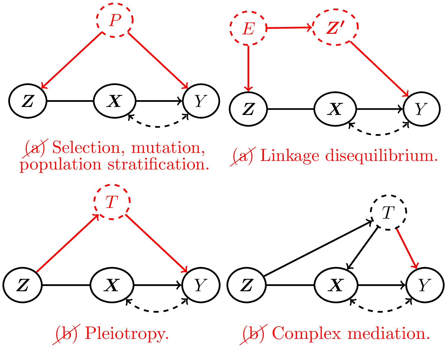
pre-treatment covariate to be a valid IV, it must be (a) unconfounded
with the outcome and (b) have a causal effect on the outcome that is
exclusively mediated by the exposure. It is impossible to test the
validity of these IV assumptions for any particular pre-treatment
covariate; however, when different pre-treatment covariates give
differing causal effect estimates if treated as IVs, then we know at
least one of the covariates violates these assumptions.
budgetIV exploits this fact by taking as input a minimum
‘’budget’’ of pre-treatment covariates assumed to be valid IVs. This can
be extended to assuming a set of budgets for varying ‘’degrees’’ of
validity set by the user and defined formally through a parameter that
captures violation of either IV assumption. These budget constraints can
be chosen using specialist knowledge or varied in a principled
sensitivity analysis. budgetIV supports non-linear
treatment effects and multi-dimensional treatments; requires only
summary statistics rather than raw data; and can be used to construct
confidence sets under a standard assumption from the Mendelian
randomisation literature. With one-dimensional \(\Phi (X)\), a computationally-efficient
variant Budget_IV_Scalar allows for use with thousands of
pre-treatment covariates.
We assume a heterogenous treatment effect, implying the following
structural causal model: \[Z := f_z
(\epsilon_z),\] \[X := f_x (Z,
\epsilon_x),\] \[Y = \theta \Phi (X) +
g_y (Z, \epsilon_y).\] There may be association between \(\epsilon_y\) and \(\epsilon_z\), indicating a violation of the
unconfoundedness assumption (a); and \(g_y\) may depend on \(Z\), indicating violation of exclusivity
(b). With budgetIV, the user defines degrees of validity
\(0 \leq \tau_1 \leq \tau_2 \leq \ldots \leq
\tau_K\) that may apply to any candidate instrument \(Z_i\). If \(Z_i\) satisfies the \(j\)’th degree of validity, this means \(\lvert \mathrm{Cov} (g_y (Z, \epsilon_y), Z_i)
\rvert \leq \tau_j\). Choosing \(\tau_1
= 0\) would demand some pre-treatment covariates give valid
causal effect estimates, while choosing \(\tau_K = \infty\) would allow for some
covariates to give arbitrarily biased causal effect estimates if treated
as IVs. budgetIV will return the corresponding
identified/confidence set over causal effects that agree with the budget
constraints and with the user-input summary statistics:
beta_y corresponding to \(\mathrm{Cov} (Y, Z)\) and
beta_Phi corresponding to \(\mathrm{Cov} (\Phi (X), Z)\). Other
regression coefficients such as odds ratios, hazard ratios or
multicolinearity-adjusted regression coefficients may be used for
beta_y and beta_Phi, but this also changes the
interpretation of the \(\tau\)’s.
For further methodological details and theoretical results and advanced use cases, please refer to Penn et al. (2024) doi:10.48550/arXiv.2411.06913.
To install the development version from GitHub, using
devtools, run:
devtools::install_github('jpenn2023/budgetivr')

library(budgetivr)First, we calculate summary statistics from the example dataset:
data(simulated_data_budgetIV)

beta_y <- simulated_data_budgetIV$beta_y

beta_phi_1 <- simulated_data_budgetIV$beta_phi_1
beta_phi_2 <- simulated_data_budgetIV$beta_phi_2

beta_phi <- matrix(c(beta_phi_1, beta_phi_2), nrow = 2, byrow = TRUE)

delta_beta_y <- simulated_data_budgetIV$delta_beta_y
Then, we define the basis functions \[\Phi (X)\] and set background budget constraints:
phi_basis <- expression(x, x^2)

tau_vec = c(0)
b_vec = c(3)
Then, we define the baseline treatment \[x_0\] and the treatment values to calculate the average treatment effect over:
X_baseline <- list("x" = c(0))

x_vals <- seq(from = 0, to = 1, length.out = 500)

ATE_search_domain <- expand.grid("x" = x_vals)
Now we run budgetIV to partially identify the budget
assignments and corresponding average causal effect bounds:
partial_identification_ATE <- budgetIV(beta_y = beta_y,
                                       beta_phi = beta_phi,
                                       phi_basis = phi_basis,
                                       tau_vec = tau_vec,
                                       b_vec = b_vec,
                                       ATE_search_domain = ATE_search_domain,
                                       X_baseline = X_baseline,
                                       delta_beta_y = delta_beta_y)