| Title: | Create, Modify and Analyse Phylogenetic Trees |
| Version: | 2.4.0 |
| License: | GPL (≥ 3) |
| Copyright: | Incorporates C/C++ code from 'ape' by Emmanuel Paradis <doi:10.1093/bioinformatics/bty633> and 'RUtreebalance' by Robert Noble <doi:10.5281/zenodo.5873857>. |
| Description: | Efficient implementations of functions for the creation, modification and analysis of phylogenetic trees. Applications include: generation of trees with specified shapes; tree rearrangement; analysis of tree shape; rooting of trees and extraction of subtrees; calculation and depiction of split support; plotting the position of rogue taxa (Klopfstein & Spasojevic 2019) <doi:10.1371/journal.pone.0212942>; calculation of ancestor-descendant relationships, of 'stemwardness' (Asher & Smith, 2022) <doi:10.1093/sysbio/syab072>, and of tree balance (Mir et al. 2013, Lemant et al. 2022) <doi:10.1016/j.mbs.2012.10.005>, <doi:10.1093/sysbio/syac027>; artificial extinction (Asher & Smith, 2022) <doi:10.1093/sysbio/syab072>; import and export of trees from Newick, Nexus (Maddison et al. 1997) <doi:10.1093/sysbio/46.4.590>, and TNT https://www.lillo.org.ar/phylogeny/tnt/ formats; and analysis of splits and cladistic information. |
| URL: | https://ms609.github.io/TreeTools/, https://github.com/ms609/TreeTools/ |
| BugReports: | https://github.com/ms609/TreeTools/issues/ |
| SystemRequirements: | C++17 |
| Depends: | R (≥ 3.6.0), ape (≥ 5.6), |
| Imports: | bit64, fastmatch (≥ 1.1.3), methods, PlotTools, Rdpack (≥ 2.6.6), |
| Suggests: | RCurl, spelling, knitr, phangorn (≥ 2.2.1), Rcpp (≥ 1.0.8), rmarkdown, testthat (≥ 3.0), TreeDist, TreeSearch, vdiffr (≥ 1.0.0), |
| Config/Needs/benchmark: | bench, TreeDist |
| Config/Needs/check: | rcmdcheck, testthat |
| Config/Needs/coverage: | covr |
| Config/Needs/memcheck: | pkgdown, testthat |
| Config/Needs/metadata: | codemeta |
| Config/Needs/revdeps: | revdepcheck |
| Config/Needs/website: | pkgdown |
| Config/roxygen2/version: | 8.0.0 |
| Config/testthat/parallel: | false |
| Config/testthat/edition: | 3 |
| LinkingTo: | Rcpp |
| RdMacros: | Rdpack |
| LazyData: | true |
| ByteCompile: | true |
| Encoding: | UTF-8 |
| Language: | en-GB |
| VignetteBuilder: | knitr |
| NeedsCompilation: | yes |
| Packaged: | 2026-06-02 15:02:39 UTC; pjjg18 |
| Author: | Martin R. Smith  [aut, cre, cph],
Emmanuel Paradis
[cph] (ape library),
Robert Noble
[cph] (RUtreebalance)
[aut, cre, cph],
Emmanuel Paradis
[cph] (ape library),
Robert Noble
[cph] (RUtreebalance) |
| Maintainer: | Martin R. Smith <martin.smith@durham.ac.uk> |
| Repository: | CRAN |
| Date/Publication: | 2026-06-02 16:50:02 UTC |
TreeTools
Description
"TreeTools" is an R package that provides functions for creating, modifying and analysing phylogenetic trees. It complements packages such as ape, phangorn and phytools, aiming for efficient and robust implementations of functions, typically applied to unweighted trees (i.e. those without edge lengths).
Details
Full documentation is available online.
Author(s)
Maintainer: Martin R. Smith martin.smith@durham.ac.uk (ORCID) [copyright holder]
Authors:
Martin R. Smith martin.smith@durham.ac.uk (ORCID) [copyright holder]
Other contributors:
Emmanuel Paradis (ORCID) (ape library) [copyright holder]
Robert Noble (ORCID) (RUtreebalance) [copyright holder]
See Also
Useful links:
Report bugs at https://github.com/ms609/TreeTools/issues/
Random parent vector
Description
Random parent vector
Usage
.RandomParent(n, seed = sample.int(2147483647L, 1L))
Arguments
n |
Integer specifying number of leaves. |
seed |
(Optional) Integer with which to seed Mersenne Twister random number generator in C++. |
Value
Integer vector corresponding to the "parent" entry of
tree[["edge"]], where the "child" entry, i.e. column 2, is numbered
sequentially from 1:n.
Author(s)
Martin R. Smith (martin.smith@durham.ac.uk)
Add a tip to a phylogenetic tree
Description
AddTip() adds a tip to a phylogenetic tree at a specified location.
Usage
AddTip(
  tree,
  where = sample.int(tree[["Nnode"]] * 2 + 2L, size = 1) - 1L,
  label = "New tip",
  nodeLabel = "",
  edgeLength = 0,
  lengthBelow = NULL,
  nTip = NTip(tree),
  nNode = tree[["Nnode"]],
  rootNode = RootNode(tree)
)

AddTipEverywhere(tree, label = "New tip", includeRoot = FALSE)
Arguments
tree |
A tree of class |
where |
The node or tip that should form the sister taxon to the new
node. To add a new tip at the root, use |
label |
Character string providing the label to apply to the new tip. |
nodeLabel |
Character string providing a label to apply to the newly
created node, if |
edgeLength |
Numeric specifying length of new edge. If |
lengthBelow |
Numeric specifying length below neighbour at which to
graft new edge. Values greater than the length of the edge will result
in negative edge lengths. If |
nTip, nNode, rootNode |
Optional integer vectors specifying number of tips
and nodes in |
includeRoot |
Logical; if |
Details
AddTip() extends bind.tree, which cannot handle
single-taxon trees.
AddTipEverywhere() adds a tip to each edge in turn.
Value
AddTip() returns a tree of class phylo with an additional tip
at the desired location.
AddTipEverywhere() returns a list of class multiPhylo containing
the trees produced by adding label to each edge of tree in turn.
Author(s)
Martin R. Smith (martin.smith@durham.ac.uk)
See Also
Add one tree to another: bind.tree()
Other tree manipulation:
CollapseNode(),
ConsensusWithout(),
DropTip(),
ImposeConstraint(),
KeptPaths(),
KeptVerts(),
LeafLabelInterchange(),
MakeTreeBinary(),
Renumber(),
RenumberTips(),
RenumberTree(),
RootTree(),
SortTree(),
Subtree(),
TipTimedTree(),
TrivialTree
Examples
tree <- BalancedTree(10)

# Add a leaf below an internal node
plot(tree)
ape::nodelabels() # Identify node numbers
node <- 15        # Select location to add leaf
ape::nodelabels(bg = ifelse(NodeNumbers(tree) == node, "green", "grey"))

plot(AddTip(tree, 15, "NEW_TIP"))

# Add edge lengths for an ultrametric tree
tree$edge.length <- rep(c(rep(1, 5), 2, 1, 2, 2), 2)

# Add a leaf to an external edge
leaf <- 5
plot(tree)
ape::tiplabels(bg = ifelse(seq_len(NTip(tree)) == leaf, "green", "grey"))

plot(AddTip(tree, 5, "NEW_TIP", edgeLength = NULL))

# Create a polytomy, rather than a new node
plot(AddTip(tree, 5, "NEW_TIP", edgeLength = NA))

# Set up multi-panel plot
oldPar <- par(mfrow = c(2, 4), mar = rep(0.3, 4), cex = 0.9)

# Add leaf to each edge on a tree in turn
backbone <- BalancedTree(4)
# Treating the position of the root as instructive:
additions <- AddTipEverywhere(backbone, includeRoot = TRUE)
xx <- lapply(additions, plot)

par(mfrow = c(2, 3))
# Don't treat root edges as distinct:
additions <- AddTipEverywhere(backbone, includeRoot = FALSE)
xx <- lapply(additions, plot)

# Restore original plotting parameters
par(oldPar)
Ancestral edge
Description
Ancestral edge
Usage
AncestorEdge(edge, parent, child)
Arguments
edge |
Number of an edge |
parent |
Integer vector corresponding to the first column of the edge
matrix of a tree of class |
child |
Integer vector corresponding to the second column of the edge
matrix of a tree of class |
Value
AncestorEdge returns a logical vector identifying whether each edge
is the immediate ancestor of the given edge.
See Also
Other tree navigation:
CladeSizes(),
DescendantEdges(),
EdgeAncestry(),
EdgeDistances(),
ListAncestors(),
MRCA(),
MatchEdges(),
NDescendants(),
NodeDepth(),
NodeNumbers(),
NodeOrder(),
PaintTree(),
RootNode()
Examples
tree <- BalancedTree(6)
parent <- tree$edge[, 1]
child <- tree$edge[, 2]
plot(tree)
ape::edgelabels()
AncestorEdge(5, parent, child)
which(AncestorEdge(5, parent, child))
Read modification time from "ape" Nexus file
Description
ApeTime() reads the time that a tree written with "ape" was modified,
based on the comment in the Nexus file.
Usage
ApeTime(filepath, format = "double")
Arguments
filepath |
Character string specifying path to the file. |
format |
Format in which to return the time: "double" as a sortable numeric;
any other value to return a string in the format
|
Value
ApeTime() returns the time that the specified file was created by
ape, in the format specified by format.
Author(s)
Martin R. Smith (martin.smith@durham.ac.uk)
Artificial Extinction
Description
Remove tokens that do not occur in a fossil "template" taxon from a living taxon, to simulate the process of fossilization in removing data from a phylogenetic dataset.
Usage
ArtificialExtinction(
  dataset,
  subject,
  template,
  replaceAmbiguous = "ambig",
  replaceCoded = "original",
  replaceAll = TRUE,
  sampleFrom = NULL
)

## S3 method for class 'matrix'
ArtificialExtinction(
  dataset,
  subject,
  template,
  replaceAmbiguous = "ambig",
  replaceCoded = "original",
  replaceAll = TRUE,
  sampleFrom = NULL
)

## S3 method for class 'phyDat'
ArtificialExtinction(
  dataset,
  subject,
  template,
  replaceAmbiguous = "ambig",
  replaceCoded = "original",
  replaceAll = TRUE,
  sampleFrom = NULL
)

ArtEx(
  dataset,
  subject,
  template,
  replaceAmbiguous = "ambig",
  replaceCoded = "original",
  replaceAll = TRUE,
  sampleFrom = NULL
)
Arguments
dataset |
Phylogenetic dataset of class |
subject |
Vector identifying subject taxa, by name or index. |
template |
Character or integer identifying taxon to use as a template. |
replaceAmbiguous, replaceCoded |
Character specifying whether tokens
that are ambiguous (
|
replaceAll |
Logical: if |
sampleFrom |
Vector identifying a subset of characters from which to
sample replacement tokens.
If |
Details
Further details are provided in Asher and Smith (2022).
Note: this simple implementation does not account for character contingency, e.g. characters whose absence imposes inapplicable or absent tokens on dependent characters.
Value
A dataset with the same class as dataset in which entries that
are ambiguous in template are made ambiguous in subject.
Author(s)
Martin R. Smith (martin.smith@durham.ac.uk)
References
Asher R, Smith MR (2022). “Phylogenetic signal and bias in paleontology.” Systematic Biology, 71(4), 986–1008. doi:10.1093/sysbio/syab072.
Examples
set.seed(1)
dataset <- matrix(c(sample(0:2, 4 * 8, TRUE),
                    "0", "0", rep("?", 6)), nrow = 5,
                    dimnames = list(c(LETTERS[1:4], "FOSSIL"),
                                    paste("char", 1:8)), byrow = TRUE)
artex <- ArtificialExtinction(dataset, c("A", "C"), "FOSSIL")
Character information content
Description
CharacterInformation() calculates the cladistic information content
(Steel and Penny 2006) of a given character, in bits.
The total information in all characters gives a measure of the potential
utility of a dataset (Cotton and Wilkinson 2008), which can be
compared with a profile parsimony score (Faith and Trueman 2001) to
evaluate the degree of homoplasy within a dataset.
Usage
CharacterInformation(tokens)
Arguments
tokens |
Character vector specifying the tokens assigned to each taxon for
a character. Example: Note that ambiguous tokens such as |
Value
CharacterInformation() returns a numeric specifying the
phylogenetic information content of the character
(sensu Steel and Penny 2006), in bits.
Author(s)
Martin R. Smith (martin.smith@durham.ac.uk)
References
Cotton JA, Wilkinson M (2008).
“Quantifying the potential utility of phylogenetic characters.”
Taxon, 57(1), 131–136.
Faith DP, Trueman JWH (2001).
“Towards an inclusive philosophy for phylogenetic inference.”
Systematic Biology, 50(3), 331–350.
doi:10.1080/10635150118627.
Steel MA, Penny D (2006).
“Maximum parsimony and the phylogenetic information in multistate characters.”
In Albert VA (ed.), Parsimony, Phylogeny, and Genomics, 163–178.
Oxford University Press, Oxford.
See Also
Other split information functions:
SplitInformation(),
SplitMatchProbability(),
TreesMatchingSplit(),
UnrootedTreesMatchingSplit()
Count cherries in a tree
Description
Cherries() counts the number of vertices in a binary tree whose children
are both leaves.
Usage
Cherries(tree, nTip)

## S3 method for class 'phylo'
Cherries(tree, nTip = NTip(tree))

## S3 method for class 'numeric'
Cherries(tree, nTip)
Arguments
tree |
A binary tree, of class |
nTip |
Number of leaves in tree. |
Value
Cherries() returns an integer specifying the number of nodes whose
children are both leaves.
Equations for the number of cherries expected under uniform and Yule tree models are derived by McKenzie and Steel (2000).
Author(s)
Martin R. Smith (martin.smith@durham.ac.uk)
References
McKenzie A, Steel M (2000). “Distributions of Cherries for Two Models of Trees.” Mathematical Biosciences, 164(1), 81–92. doi:10.1016/S0025-5564(99)00060-7.
See Also
Other tree properties:
ConsensusWithout(),
EdgeRatio(),
LongBranch(),
MatchEdges(),
NSplits(),
NTip(),
NodeNumbers(),
PathLengths(),
SplitsInBinaryTree(),
TipLabels(),
TreeIsRooted(),
Treeness()
Clade sizes
Description
CladeSizes() reports the number of nodes in each clade in a tree.
Usage
CladeSizes(tree, internal = FALSE, nodes = NULL)
Arguments
tree |
A tree of class |
internal |
Logical specifying whether internal nodes should be counted towards the size of each clade. |
nodes |
Integer specifying indices of nodes at the base of clades whose sizes should be returned. If unspecified, counts will be provided for all nodes (including leaves). |
Value
CladeSizes() returns the number of nodes (including leaves) that
are descended from each node, not including the node itself.
See Also
Other tree navigation:
AncestorEdge(),
DescendantEdges(),
EdgeAncestry(),
EdgeDistances(),
ListAncestors(),
MRCA(),
MatchEdges(),
NDescendants(),
NodeDepth(),
NodeNumbers(),
NodeOrder(),
PaintTree(),
RootNode()
Examples
tree <- BalancedTree(6)
plot(tree)
ape::nodelabels()
CladeSizes(tree, nodes = c(1, 8, 9))
Cladistic information content of a tree
Description
CladisticInfo() calculates the cladistic (phylogenetic) information
content of a phylogenetic object, sensu Thorley et al. (1998).
Usage
CladisticInfo(x)

## S3 method for class 'phylo'
CladisticInfo(x)

## S3 method for class 'Splits'
CladisticInfo(x)

## S3 method for class 'list'
CladisticInfo(x)

## S3 method for class 'multiPhylo'
CladisticInfo(x)

CladisticInformation(x)
Arguments
x |
Tree of class |
Details
The CIC is the logarithm of the number of binary trees that include the specified topology. A base two logarithm gives an information content in bits.
The CIC was originally proposed by Rohlf (1982), and formalised, with an information-theoretic justification, by Thorley et al. (1998). Steel and Penny (2006) term the equivalent quantity "phylogenetic information content" in the context of individual characters.
The number of binary trees consistent with a cladogram provides a more satisfactory measure of the resolution of a tree than simply counting the number of edges resolved (Page 1992).
Value
CladisticInfo() returns a numeric giving the cladistic information
content of the input tree(s), in bits.
If passed a Splits object, it returns the information content of each
split in turn.
Author(s)
Martin R. Smith (martin.smith@durham.ac.uk)
References
Page RD (1992).
“Comments on the information content of classifications.”
Cladistics, 8(1), 87–95.
doi:10.1111/j.1096-0031.1992.tb00054.x.
Rohlf FJ (1982).
“Consensus indices for comparing classifications.”
Mathematical Biosciences, 59(1), 131–144.
doi:10.1016/0025-5564(82)90112-2.
Steel MA, Penny D (2006).
“Maximum parsimony and the phylogenetic information in multistate characters.”
In Albert VA (ed.), Parsimony, Phylogeny, and Genomics, 163–178.
Oxford University Press, Oxford.
Thorley JL, Wilkinson M, Charleston M (1998).
“The information content of consensus trees.”
In Rizzi A, Vichi M, Bock H (eds.), Advances in Data Science and Classification, 91–98.
Springer, Berlin.
ISBN 978-3-540-64641-9.
doi:10.1007/978-3-642-72253-0.
See Also
Other tree information functions:
NRooted(),
TreesMatchingTree()
Other tree characterization functions:
Consensus(),
J1Index(),
Stemwardness,
TotalCopheneticIndex()
Convert phylogenetic tree to ClusterTable
Description
as.ClusterTable() converts a phylogenetic tree to a ClusterTable object,
which is an internal representation of its splits suitable for rapid tree
distance calculation (per Day, 1985).
Usage
as.ClusterTable(x, tipLabels = NULL, ...)

## S3 method for class 'phylo'
as.ClusterTable(x, tipLabels = NULL, ...)

## S3 method for class 'list'
as.ClusterTable(x, tipLabels = NULL, ...)

## S3 method for class 'multiPhylo'
as.ClusterTable(x, tipLabels = NULL, ...)
Arguments
x |
Object to convert into |
tipLabels |
Character vector specifying sequence in which to order tip labels. |
... |
Unused. |
Details
Each row of a cluster table relates to a clade on a tree rooted on tip 1.
Tips are numbered according to the order in which they are visited in
preorder: i.e., if plotted using plot(x), from the top of the page
downwards. A clade containing the tips 2 .. 5 would be denoted by the
entry 2, 5, in either row 2 or row 5 of the cluster table.
Value
as.ClusterTable() returns an object of class ClusterTable,
or a list thereof.
Author(s)
Martin R. Smith (martin.smith@durham.ac.uk)
References
Day WHE (1985). “Optimal algorithms for comparing trees with labeled leaves.” Journal of Classification, 2(1), 7–28. doi:10.1007/BF01908061.
See Also
S3 methods for ClusterTable objects.
Other utility functions:
ClusterTable-methods,
Hamming(),
MSTEdges(),
SampleOne(),
TipTimedTree(),
UnshiftTree(),
as.multiPhylo(),
match,phylo,phylo-method,
sapply64(),
sort.multiPhylo()
Examples
tree1 <- ape::read.tree(text = "(A, (B, (C, (D, E))));");
tree2 <- ape::read.tree(text = "(A, (B, (D, (C, E))));");
ct1 <- as.ClusterTable(tree1)
summary(ct1)
as.matrix(ct1)

# Tip label order must match ct1 to allow comparison
ct2 <- as.ClusterTable(tree2, tipLabels = LETTERS[1:5])

# It can thus be safer to use
ctList <- as.ClusterTable(c(tree1, tree2))
ctList[[2]]
S3 methods for ClusterTable objects
Description
S3 methods for ClusterTable objects.
Usage
## S3 method for class 'ClusterTable'
as.matrix(x, ...)

## S3 method for class 'ClusterTable'
print(x, ...)

## S3 method for class 'ClusterTable'
summary(object, ...)
Arguments
x, object |
Object of class |
... |
Additional arguments for consistency with S3 methods. |
Author(s)
Martin R. Smith (martin.smith@durham.ac.uk)
See Also
Other utility functions:
ClusterTable,
Hamming(),
MSTEdges(),
SampleOne(),
TipTimedTree(),
UnshiftTree(),
as.multiPhylo(),
match,phylo,phylo-method,
sapply64(),
sort.multiPhylo()
Examples
clustab <- as.ClusterTable(TreeTools::BalancedTree(6))
as.matrix(clustab)
print(clustab)
summary(clustab)
Collapse nodes on a phylogenetic tree
Description
Collapses specified nodes or edges on a phylogenetic tree, resulting in polytomies.
Usage
CollapseNode(tree, nodes)

## S3 method for class 'phylo'
CollapseNode(tree, nodes)

CollapseEdge(tree, edges)
Arguments
tree |
A tree of class |
nodes, edges |
Integer vector specifying the nodes or edges in the tree
to be dropped.
(Use |
Value
CollapseNode() and CollapseEdge() return a tree of class phylo,
corresponding to tree with the specified nodes or edges collapsed.
The length of each dropped edge will (naively) be added to each descendant
edge.
Author(s)
Martin R. Smith
See Also
Other tree manipulation:
AddTip(),
ConsensusWithout(),
DropTip(),
ImposeConstraint(),
KeptPaths(),
KeptVerts(),
LeafLabelInterchange(),
MakeTreeBinary(),
Renumber(),
RenumberTips(),
RenumberTree(),
RootTree(),
SortTree(),
Subtree(),
TipTimedTree(),
TrivialTree
Examples
oldPar <- par(mfrow = c(3, 1), mar = rep(0.5, 4))

tree <- as.phylo(898, 7)
tree$edge.length <- 11:22
plot(tree)
nodelabels()
edgelabels()
edgelabels(round(tree$edge.length, 2),
           cex = 0.6, frame = "n", adj = c(1, -1))

# Collapse by node number
newTree <- CollapseNode(tree, c(12, 13))
plot(newTree)
nodelabels()
edgelabels(round(newTree$edge.length, 2),
           cex = 0.6, frame = "n", adj = c(1, -1))

# Collapse by edge number
newTree <- CollapseEdge(tree, c(2, 4))
plot(newTree)

par(oldPar)
Which splits are compatible?
Description
Which splits are compatible?
Usage
CompatibleSplits(splits, splits2)

.CompatibleSplit(a, b, nTip)

.CompatibleRaws(rawA, rawB, bitmask)
Arguments
splits |
An object of class |
splits2 |
A second |
a, b |
Raw representations of splits, from a row of a |
rawA, rawB |
Raw representations of splits. |
bitmask |
Raw masking bits that do not correspond to tips. |
Value
CompatibleSplits returns a logical matrix specifying whether each
split in splits is compatible with each split in splits2.
.CompatibleSplit returns a logical vector stating whether splits
are compatible.
.CompatibleRaws returns a logical vector specifying whether input
raws are compatible.
Author(s)
Martin R. Smith (martin.smith@durham.ac.uk)
Examples
splits <- as.Splits(BalancedTree(8))
splits2 <- as.Splits(PectinateTree(8))

summary(splits)
summary(splits2)

CompatibleSplits(splits, splits2)
Construct consensus trees
Description
Consensus() calculates the majority-rule or strict consensus of a set of
trees, using the cluster-table approach of (Day 1985).
Usage
Consensus(trees, p = 1, check.labels = TRUE, hash = TRUE)
Arguments
trees |
List of trees, optionally of class |
p |
Proportion of trees that must contain a split for it to be reported
in the consensus. |
check.labels |
Logical specifying whether to check that all trees have
identical labels. Defaults to |
hash |
Logical; if |
Details
The strict consensus (p = 1) compares the clusters of the first tree
against every other tree in linear time. The majority-rule and threshold
consensus (0.5 <= p < 1) instead count the frequency of every split across
all trees in a single pass and retain those occurring in a proportion p or
more of trees; this runs in time linear in the number of trees, after
(Jansson et al. 2016). By default the count uses
a 128-bit hash, whose results are exact with overwhelming probability; set
hash = FALSE for a slower but guaranteed-exact count.
Value
Consensus() returns an object of class phylo, rooted as in the
first entry of trees.
Author(s)
Martin R. Smith (martin.smith@durham.ac.uk)
References
Day WHE (1985).
“Optimal algorithms for comparing trees with labeled leaves.”
Journal of Classification, 2(1), 7–28.
doi:10.1007/BF01908061.
Jansson J, Shen C, Sung W (2016).
“Improved algorithms for constructing consensus trees.”
Journal of the ACM, 63(3), 28:1–28:24.
doi:10.1145/2898436.
See Also
-
ConsTree implements other consensus tree algorithms.
-
Rogue increases the resolution of consensus trees by dropping wildcard taxa.
-
TreeDist::ConsensusInfo()calculates the information content of a consensus tree.
Other consensus tree functions:
ConsensusWithout(),
RoguePlot()
Other tree characterization functions:
CladisticInfo(),
J1Index(),
Stemwardness,
TotalCopheneticIndex()
Examples
Consensus(as.phylo(0:2, 8))
Reduced consensus, omitting specified taxa
Description
ConsensusWithout() displays a consensus plot with specified taxa excluded,
which can be a useful way to increase the resolution of a consensus tree
when a few wildcard taxa obscure a consistent set of relationships.
MarkMissing() adds missing taxa as loose leaves on the plot.
Usage
ConsensusWithout(trees, tip = character(0), ...)

## S3 method for class 'phylo'
ConsensusWithout(trees, tip = character(0), ...)

## S3 method for class 'multiPhylo'
ConsensusWithout(trees, tip = character(0), ...)

## S3 method for class 'list'
ConsensusWithout(trees, tip = character(0), ...)

MarkMissing(tip, position = "bottomleft", ...)
Arguments
trees |
A list of phylogenetic trees, of class |
tip |
A character vector specifying the names (or numbers) of tips to
drop (using |
... |
Additional parameters to pass on to |
position |
Where to plot the missing taxa.
See |
Value
ConsensusWithout() returns a consensus tree (of class phylo)
without the excluded taxa.
MarkMissing() provides a null return, after plotting the specified
tips as a legend.
Author(s)
Martin R. Smith (martin.smith@durham.ac.uk)
See Also
Other tree manipulation:
AddTip(),
CollapseNode(),
DropTip(),
ImposeConstraint(),
KeptPaths(),
KeptVerts(),
LeafLabelInterchange(),
MakeTreeBinary(),
Renumber(),
RenumberTips(),
RenumberTree(),
RootTree(),
SortTree(),
Subtree(),
TipTimedTree(),
TrivialTree
Other tree properties:
Cherries(),
EdgeRatio(),
LongBranch(),
MatchEdges(),
NSplits(),
NTip(),
NodeNumbers(),
PathLengths(),
SplitsInBinaryTree(),
TipLabels(),
TreeIsRooted(),
Treeness()
Other consensus tree functions:
Consensus(),
RoguePlot()
Examples
oldPar <- par(mfrow = c(1, 2), mar = rep(0.5, 4))

# Two trees differing only in placement of tip 2:
trees <- as.phylo(c(0, 53), 6)
plot(trees[[1]])
plot(trees[[2]])

# Strict consensus (left panel) lacks resolution:
plot(ape::consensus(trees))

# But omitting tip two (right panel) reveals shared structure in common:
plot(ConsensusWithout(trees, "t2"))
MarkMissing("t2")

par(oldPar)
Constrained neighbour-joining tree
Description
Constructs an approximation to a neighbour-joining tree, modified in order to be consistent with a constraint. Zero-length branches are collapsed at random.
Usage
ConstrainedNJ(dataset, constraint, weight = 1L, ratio = TRUE, ambig = "mean")
Arguments
dataset |
A phylogenetic data matrix of phangorn class |
constraint |
Either an object of class |
weight |
Numeric specifying degree to up-weight characters in
|
ambig, ratio |
Settings of |
Value
ConstrainedNJ() returns a tree of class phylo.
Author(s)
Martin R. Smith (martin.smith@durham.ac.uk)
See Also
Other tree generation functions:
GenerateTree,
NJTree(),
TreeNumber,
TrivialTree
Examples
dataset <- MatrixToPhyDat(matrix(
  c(0, 1, 1, 1, 0, 1,
    0, 1, 1, 0, 0, 1), ncol = 2,
  dimnames = list(letters[1:6], NULL)))
constraint <- MatrixToPhyDat(
  c(a = 0, b = 0, c = 0, d = 0, e = 1, f = 1))
plot(ConstrainedNJ(dataset, constraint))
Decompose additive (ordered) phylogenetic characters
Description
Decompose() decomposes additive characters into a series of binary
characters, which is mathematically equivalent when analysed under
equal weights parsimony. (This equivalence is not exact
under implied weights or under probabilistic tree inference methods.)
Usage
Decompose(dataset, indices)
Arguments
dataset |
A phylogenetic data matrix of phangorn class |
indices |
Integer or logical vector specifying indices of characters that should be decomposed |
Details
An ordered (additive) character can be rewritten as a mathematically equivalent hierarchy of binary neomorphic characters (Farris et al. 1970). Two reasons to prefer the latter approach are:
It makes explicit the evolutionary assumptions underlying an ordered character, whether the underlying ordering is linear, reticulate or branched (Mabee 1989).
It avoids having to identify characters requiring special treatment to phylogenetic software, which requires the maintenance of an up-to-date log of which characters are treated as additive and which sequence their states occur in, a step that may be overlooked by re-users of the data.
Careful consideration is warranted when evaluating whether a group of related characteristics ought to be treated as ordered (Wilkinson 1992). On the one hand, the 'principle of indifference' states that we should treat all transformations as equally probable (/ surprising / informative); ordered characters fail this test, as larger changes are treated as less probable than smaller ones. On the other hand, ordered characters allow more opportunities for homology of different character states, and might thus be defended under the auspices of Hennig's Auxiliary Principle (Wilkinson 1992).
For a case study of how ordering phylogenetic characters can affect phylogenetic outcomes in practice, see Brady et al. (2024).
Value
Decompose() returns a phyDat object in which the specified
ordered characters have been decomposed into binary characters.
The attribute originalIndex lists the index of the character in
dataset to which each element corresponds.
Author(s)
Martin R. Smith (martin.smith@durham.ac.uk)
References
Brady PL, Castrellon Arteaga A, López-Torres S, Springer MS (2024).
“The Effects of Ordered Multistate Morphological Characters on Phylogenetic Analyses of Eutherian Mammals.”
Journal of Mammalian Evolution, 31(3), 28.
doi:10.1007/s10914-024-09727-2.
Farris JS, Kluge AG, Eckardt MJ (1970).
“A Numerical Approach to Phylogenetic Systematics.”
Systematic Biology, 19(2), 172–189.
doi:10.2307/2412452.
Mabee PM (1989).
“Assumptions Underlying the Use of Ontogenetic Sequences for Determining Character State Order.”
Transactions of the American Fisheries Society, 118(2), 151–158.
doi:10.1577/1548-8659(1989)118<0151:AUTUOO>2.3.CO;2.
Wilkinson M (1992).
“Ordered versus Unordered Characters.”
Cladistics, 8(4), 375–385.
doi:10.1111/j.1096-0031.1992.tb00079.x.
See Also
Other phylogenetic matrix conversion functions:
MatrixToPhyDat(),
NexusTokensToInteger(),
Reweight(),
StringToPhyDat()
Examples
data("Lobo")

# Identify character 11 as additive
# Character 11 will be replaced with two characters
# The present codings 0, 1 and 2 will be replaced with 00, 10, and 11.
decomposed <- Decompose(Lobo.phy, 11)

NumberOfChars <- function(x) sum(attr(x, "weight"))
NumberOfChars(Lobo.phy)   # 115 characters in original
NumberOfChars(decomposed) # 116 characters in decomposed
Identify descendant edges
Description
DescendantEdges() efficiently identifies edges that are "descended" from
edges in a tree.
DescendantTips() efficiently identifies leaves (external nodes) that are
"descended" from edges in a tree.
Usage
DescendantEdges(
  parent,
  child,
  edge = NULL,
  node = NULL,
  nEdge = length(parent),
  includeSelf = TRUE
)

DescendantTips(parent, child, edge = NULL, node = NULL, nEdge = length(parent))
Arguments
parent |
Integer vector corresponding to the first column of the edge
matrix of a tree of class |
child |
Integer vector corresponding to the second column of the edge
matrix of a tree of class |
edge |
Integer specifying the number of the edge whose children are
required (see |
node |
Integer specifying the number(s) of nodes whose children are
required. Specify |
nEdge |
number of edges (calculated from |
includeSelf |
Logical specifying whether to mark |
Value
DescendantEdges() returns a logical vector stating whether each
edge in turn is the specified edge (if includeSelf = TRUE)
or one of its descendants.
DescendantTips() returns a logical vector stating whether each
leaf in turn is a descendant of the specified edge.
See Also
Other tree navigation:
AncestorEdge(),
CladeSizes(),
EdgeAncestry(),
EdgeDistances(),
ListAncestors(),
MRCA(),
MatchEdges(),
NDescendants(),
NodeDepth(),
NodeNumbers(),
NodeOrder(),
PaintTree(),
RootNode()
Examples
tree <- as.phylo(0, 6)
plot(tree)
desc <- DescendantEdges(tree$edge[, 1], tree$edge[, 2], edge = 5)
which(desc)
ape::edgelabels(bg = 3 + desc)
tips <- DescendantTips(tree$edge[, 1], tree$edge[, 2], edge = 5)
which(tips)
tiplabels(bg = 3 + tips)
Double factorial
Description
Calculate the double factorial of a number, or its logarithm.
Usage
DoubleFactorial(n)

DoubleFactorial64(n)

LnDoubleFactorial(n)

Log2DoubleFactorial(n)

LogDoubleFactorial(n)

LnDoubleFactorial.int(n)

LogDoubleFactorial.int(n)
Arguments
n |
Vector of integers. |
Value
Returns the double factorial, n * (n - 2) * (n - 4) * (n - 6) * ...
Functions
-
DoubleFactorial64(): Returns the exact double factorial as a 64-bitinteger64, forn< 34. -
LnDoubleFactorial(): Returns the logarithm of the double factorial. -
Log2DoubleFactorial(): Returns the logarithm of the double factorial. -
LnDoubleFactorial.int(): Slightly faster, when x is known to be length one and below 50001
Author(s)
Martin R. Smith (martin.smith@durham.ac.uk)
See Also
Other double factorials:
doubleFactorials,
logDoubleFactorials
Examples
DoubleFactorial (-4:0) # Return 1 if n < 2
DoubleFactorial (2) # 2
DoubleFactorial (5) # 1 * 3 * 5
exp(LnDoubleFactorial.int (8)) # log(2 * 4 * 6 * 8)
DoubleFactorial64(31)
Drop leaves from tree
Description
DropTip() removes specified leaves from a phylogenetic tree, collapsing
incident branches.
Usage
DropTip(tree, tip, preorder = TRUE, check = TRUE)

KeepTip(tree, tip, preorder = TRUE, check = TRUE)

## S3 method for class 'phylo'
DropTip(tree, tip, preorder = TRUE, check = TRUE)

## S3 method for class 'phylo'
KeepTip(tree, tip, preorder = TRUE, check = TRUE)

## S3 method for class 'Splits'
KeepTip(tree, tip, preorder = TRUE, check = TRUE)

## S3 method for class 'Splits'
DropTip(tree, tip, preorder, check = TRUE)

DropTipPhylo(tree, tip, preorder = TRUE, check = TRUE)

## S3 method for class 'multiPhylo'
DropTip(tree, tip, preorder = TRUE, check = TRUE)

## S3 method for class 'multiPhylo'
KeepTip(tree, tip, preorder = TRUE, check = TRUE)

## S3 method for class 'list'
DropTip(tree, tip, preorder = TRUE, check = TRUE)

## S3 method for class 'list'
KeepTip(tree, tip, preorder = TRUE, check = TRUE)

## S3 method for class ''NULL''
DropTip(tree, tip, preorder = TRUE, check = TRUE)

## S3 method for class ''NULL''
KeepTip(tree, tip, preorder = TRUE, check = TRUE)

KeepTipPreorder(tree, tip)

KeepTipPostorder(tree, tip)
Arguments
tree |
A tree of class |
tip |
Character vector specifying labels of leaves in tree to be dropped or kept, or integer vector specifying the indices of leaves to be dropped or kept. Specifying the index of an internal node will drop all descendants of that node. |
preorder |
Logical specifying whether to Preorder |
check |
Logical specifying whether to check validity of |
Details
This function differs from ape::drop.tip(), which roots unrooted trees,
and which can crash when trees' internal numbering follows unexpected schema.
Value
DropTip() returns a tree of class phylo, with the requested
leaves removed. The edges of the tree will be numbered in preorder,
but their sequence may not conform to the conventions of Preorder().
KeepTip() returns tree with all leaves not in tip removed,
in preorder.
Functions
-
DropTipPhylo(): Direct call toDropTip.phylo(), to avoid overhead of querying object's class. -
KeepTipPreorder(): Faster version with no checks. Does not retain labels or edge weights. Edges must be listed in preorder. May crash if improper input is specified. -
KeepTipPostorder(): Faster version with no checks. Does not retain labels or edge weights. Edges must be listed in postorder. May crash if improper input is specified.
Author(s)
Martin R. Smith (martin.smith@durham.ac.uk)
See Also
Other tree manipulation:
AddTip(),
CollapseNode(),
ConsensusWithout(),
ImposeConstraint(),
KeptPaths(),
KeptVerts(),
LeafLabelInterchange(),
MakeTreeBinary(),
Renumber(),
RenumberTips(),
RenumberTree(),
RootTree(),
SortTree(),
Subtree(),
TipTimedTree(),
TrivialTree
Other split manipulation functions:
SplitConsistent(),
Subsplit(),
TrivialSplits()
Examples
tree <- BalancedTree(9)
plot(tree)
plot(DropTip(tree, c("t5", "t6")))

unrooted <- UnrootTree(tree)
plot(unrooted)
plot(DropTip(unrooted, 4:5))

summary(DropTip(as.Splits(tree), 4:5))
Ancestors of an edge
Description
Quickly identify edges that are "ancestral" to a particular edge in a tree.
Usage
EdgeAncestry(edge, parent, child, stopAt = (parent == min(parent)))
Arguments
edge |
Integer specifying the number of the edge whose child edges should be returned. |
parent |
Integer vector corresponding to the first column of the edge
matrix of a tree of class |
child |
Integer vector corresponding to the second column of the edge
matrix of a tree of class |
stopAt |
Integer or logical vector specifying the edge(s) at which to terminate the search; defaults to the edges with the smallest parent, which will be the root edges if nodes are numbered Cladewise or in Preorder. |
Value
EdgeAncestry() returns a logical vector stating whether each edge
in turn is a descendant of the specified edge.
Author(s)
Martin R. Smith (martin.smith@durham.ac.uk)
See Also
Other tree navigation:
AncestorEdge(),
CladeSizes(),
DescendantEdges(),
EdgeDistances(),
ListAncestors(),
MRCA(),
MatchEdges(),
NDescendants(),
NodeDepth(),
NodeNumbers(),
NodeOrder(),
PaintTree(),
RootNode()
Examples
tree <- PectinateTree(6)
plot(tree)
ape::edgelabels()
parent <- tree$edge[, 1]
child <- tree$edge[, 2]
EdgeAncestry(7, parent, child)
which(EdgeAncestry(7, parent, child, stopAt = 4))
Distance between edges
Description
Number of nodes that must be traversed to navigate from each edge to each other edge within a tree
Usage
EdgeDistances(tree)
Arguments
tree |
A tree of class |
Value
EdgeDistances() returns a symmetrical matrix listing the number
of edges that must be traversed to travel from each numbered edge to each
other.
The two edges straddling the root of a rooted tree
are treated as a single edge. Add a "root" tip using AddTip() if the
position of the root is significant.
Author(s)
Martin R. Smith (martin.smith@durham.ac.uk)
See Also
Other tree navigation:
AncestorEdge(),
CladeSizes(),
DescendantEdges(),
EdgeAncestry(),
ListAncestors(),
MRCA(),
MatchEdges(),
NDescendants(),
NodeDepth(),
NodeNumbers(),
NodeOrder(),
PaintTree(),
RootNode()
Examples
tree <- BalancedTree(5)
plot(tree)
ape::edgelabels()

EdgeDistances(tree)
Ratio of external:internal edge length
Description
Reports the ratio of tree length associated with external edges (i.e. edges whose child is a leaf) and internal edges. Where tree length is dominated by internal edges, variation between tips is dominantly controlled by phylogenetic history.
Usage
EdgeRatio(x)

## S3 method for class 'phylo'
EdgeRatio(x)
Arguments
x |
A tree of class |
Value
EdgeRatio() returns a numeric specifying the ratio of external
to internal edge length (> 1 means the length of a tree is predominantly
in external edges), with attributes external, internal, and total
specifying the total length associated with edges of that nature.
Author(s)
Martin R. Smith (martin.smith@durham.ac.uk)
See Also
Other tree properties:
Cherries(),
ConsensusWithout(),
LongBranch(),
MatchEdges(),
NSplits(),
NTip(),
NodeNumbers(),
PathLengths(),
SplitsInBinaryTree(),
TipLabels(),
TreeIsRooted(),
Treeness()
Add full stop to end of a sentence
Description
Add full stop to end of a sentence
Usage
EndSentence(string)
Arguments
string |
Input string |
Value
EndSentence() returns string, punctuated with a final full stop
(period).'
Author(s)
Martin R. Smith
See Also
Other string parsing functions:
MatchStrings(),
MorphoBankDecode(),
RightmostCharacter(),
Unquote()
Examples
EndSentence("Hello World") # "Hello World."
Extract taxa from a matrix block
Description
Extract leaf labels and character states from a Nexus-formatted matrix.
Usage
ExtractTaxa(matrixLines, character_num = NULL, continuous = FALSE)

NexusTokens(tokens, character_num = NULL)
Arguments
matrixLines |
Character vector containing lines of a file that include
a phylogenetic matrix. See |
character_num |
Index of character(s) to return.
|
continuous |
Logical specifying whether characters are continuous.
Treated as discrete if |
tokens |
Vector of character strings corresponding to phylogenetic tokens. |
Value
ExtractTaxa() returns a matrix with n rows, each named for the
relevant taxon, and c columns,
each corresponding to the respective character specified in character_num.
NexusTokens() returns a character vector in which each entry
corresponds to the states of a phylogenetic character, or a list containing
an error message if input is invalid.
Examples
fileName <- paste0(system.file(package = "TreeTools"),
                   "/extdata/input/dataset.nex")
matrixLines <- readLines(fileName)[6:11]
ExtractTaxa(matrixLines)

NexusTokens("01[01]-?")
Generate pectinate, balanced or random trees
Description
RandomTree(), PectinateTree(), BalancedTree() and StarTree()
generate trees with the specified shapes and leaf labels.
Usage
RandomTree(tips, root = FALSE, nodes, lengths = NULL)

YuleTree(tips, addInTurn = FALSE, root = TRUE, lengths = NULL)

PectinateTree(tips, lengths = NULL)

BalancedTree(tips, lengths = NULL)

StarTree(tips, lengths = NULL)
Arguments
tips |
An integer specifying the number of tips, or a character vector
naming the tips, or any other object from which |
root |
Character or integer specifying tip to use as root;
or |
nodes |
Number of nodes to generate. The default and maximum,
|
lengths |
Numeric vector of edge lengths, or a function that returns
such a vector when passed the number of edges as its argument (e.g. |
addInTurn |
Logical specifying whether to add leaves in the order of
|
Value
Each function returns an unweighted binary tree of class phylo with
the specified leaf labels. Trees are rooted unless root = FALSE.
RandomTree() returns a topology drawn at random from the uniform
distribution (i.e. each binary tree is drawn with equal probability).
Trees are generated by inserting
each tip in term at a randomly selected edge in the tree.
Random numbers are generated using a Mersenne Twister.
If root = FALSE, the tree will be unrooted, with the first tip in a
basal position. Otherwise, the tree will be rooted on root.
YuleTree() returns a topology generated by the Yule process
(Steel and McKenzie 2001),
i.e. adding leaves in turn adjacent to a randomly-chosen existing leaf.
PectinateTree() returns a pectinate (caterpillar) tree.
BalancedTree() returns a balanced (symmetrical) tree, in preorder.
StarTree() returns a completely unresolved (star) tree.
Author(s)
Martin R. Smith (martin.smith@durham.ac.uk)
References
Steel MA, McKenzie A (2001). “Properties of Phylogenetic Trees Generated by Yule-type Speciation Models.” Mathematical Biosciences, 170(1), 91–112. doi:10.1016/S0025-5564(00)00061-4.()
See Also
Other tree generation functions:
ConstrainedNJ(),
NJTree(),
TreeNumber,
TrivialTree
Examples
# Set random seed for reproducibility
set.seed(10)

# Generate a tree from a phylogenetic dataset
data("Lobo")
RandomTree(Lobo.phy, lengths = runif)

# Generate trees on letters A-J
plot(RandomTree(LETTERS[1:10], root = TRUE))

plot(YuleTree(LETTERS[1:10]))

plot(PectinateTree(LETTERS[1:10]))

plot(BalancedTree(LETTERS[1:10], lengths = 1:18))

plot(StarTree(LETTERS[1:10]))
Hamming distance between taxa in a phylogenetic dataset
Description
The Hamming distance between a pair of taxa is the number of characters with a different coding, i.e. the smallest number of evolutionary steps that must have occurred since their common ancestor.
Usage
Hamming(
  dataset,
  ratio = TRUE,
  ambig = c("median", "mean", "zero", "one", "na", "nan")
)
Arguments
dataset |
Object of class |
ratio |
Logical specifying whether to weight distance against maximum possible, given that a token that is ambiguous in either of two taxa cannot contribute to the total distance between the pair. |
ambig |
Character specifying value to return when a pair of taxa
have a zero maximum distance (perhaps due to a preponderance of ambiguous
tokens).
"median", the default, take the median of all other distance values;
"mean", the mean;
"zero" sets to zero; "one" to one;
"NA" to |
Details
Tokens that contain the inapplicable state are treated as requiring no steps to transform into any applicable token.
Value
Hamming() returns an object of class dist listing the Hamming
distance between each pair of taxa.
Author(s)
Martin R. Smith (martin.smith@durham.ac.uk)
See Also
Used to construct neighbour joining trees in NJTree().
dist.hamming() in the phangorn package provides an alternative
implementation.
Other utility functions:
ClusterTable,
ClusterTable-methods,
MSTEdges(),
SampleOne(),
TipTimedTree(),
UnshiftTree(),
as.multiPhylo(),
match,phylo,phylo-method,
sapply64(),
sort.multiPhylo()
Examples
tokens <- matrix(c(0, 0, "0", 0, "?",
                   0, 0, "1", 0, 1,
                   0, 0, "1", 0, 1,
                   0, 0, "2", 0, 1,
                   1, 1, "-", "?", 0,
                   1, 1, "2", 1, "{01}"),
                   nrow = 6, ncol = 5, byrow = TRUE,
                   dimnames = list(
                     paste0("Taxon_", LETTERS[1:6]),
                     paste0("Char_", 1:5)))

dataset <- MatrixToPhyDat(tokens)
Hamming(dataset)
Force a tree to match a constraint
Description
Modify a tree such that it matches a specified constraint.
This is at present a somewhat crude implementation that attempts to retain
much of the structure of tree whilst guaranteeing compatibility with
each entry in constraint.
Usage
ImposeConstraint(tree, constraint)

AddUnconstrained(constraint, toAdd, asPhyDat = TRUE)
Arguments
tree |
A tree of class |
constraint |
Either an object of class |
toAdd |
Character vector specifying taxa to add to constraint. |
asPhyDat |
Logical: if |
Value
ImposeConstraint() returns a tree of class phylo, consistent
with constraint.
Functions
-
AddUnconstrained(): Expand a constraint to include unconstrained taxa.
Author(s)
Martin R. Smith (martin.smith@durham.ac.uk)
See Also
Other tree manipulation:
AddTip(),
CollapseNode(),
ConsensusWithout(),
DropTip(),
KeptPaths(),
KeptVerts(),
LeafLabelInterchange(),
MakeTreeBinary(),
Renumber(),
RenumberTips(),
RenumberTree(),
RootTree(),
SortTree(),
Subtree(),
TipTimedTree(),
TrivialTree
Examples
tips <- letters[1:9]
tree <- as.phylo(1, 9, tips)
plot(tree)

constraint <- StringToPhyDat("0000?1111 000111111 0000??110", tips, FALSE)
plot(ImposeConstraint(tree, constraint))
Robust universal tree balance index
Description
Calculate tree balance index J1
(when nonRootDominance = FALSE) or
J1c
(when nonRootDominance = TRUE) from (Lemant et al. 2022).
Usage
J1Index(tree, q = 1, nonRootDominance = FALSE)

JQIndex(tree, q = 1, nonRootDominance = FALSE)
Arguments
tree |
Either an object of class 'phylo', or a dataframe with column
names Parent, Identity and (optionally) Population.
The latter is similar to |
q |
Numeric between zero and one specifying sensitivity to type
frequencies. If |
nonRootDominance |
Logical specifying whether to use non-root dominance factor. |
Details
If population sizes are not provided, then the function assigns size 0 to internal nodes, and size 1 to leaves.
Value
J1Index() returns a numeric specifying the
J1 index of tree.
J^1(T) = 1 for a perfectly balanced tree;
J^1(T) = 0 for a pectinate (linear / caterpillar) tree.
Author(s)
Rob Noble, adapted by Martin R. Smith
References
Lemant J, Le Sueur C, Manojlović V, Noble R (2022). “Robust, Universal Tree Balance Indices.” Systematic Biology, 71(5), 1210–1224. doi:10.1093/sysbio/syac027.
See Also
Other tree characterization functions:
CladisticInfo(),
Consensus(),
Stemwardness,
TotalCopheneticIndex()
Examples
# Using phylo object as input:
phylo_tree <- read.tree(text="((a:0.1)A:0.5,(b1:0.2,b2:0.1)B:0.2);")
J1Index(phylo_tree)
phylo_tree2 <- read.tree(text='((A, B), ((C, D), (E, F)));')
J1Index(phylo_tree2)

# Using edges lists as input:
tree1 <- data.frame(Parent = c(1, 1, 1, 1, 2, 3, 4),
                    Identity = 1:7,
                    Population = c(1, rep(5, 6)))
J1Index(tree1)
tree2 <- data.frame(Parent = c(1, 1, 1, 1, 2, 3, 4),
                    Identity = 1:7,
                    Population = c(rep(0, 4), rep(1, 3)))
J1Index(tree2)
tree3 <- data.frame(Parent = c(1, 1, 1, 1, 2, 3, 4),
                    Identity = 1:7,
                    Population = c(0, rep(1, 3), rep(0, 3)))
J1Index(tree3)
cat_tree <- data.frame(Parent = c(1, 1:14, 1:15, 15),
                       Identity = 1:31,
                       Population = c(rep(0, 15), rep(1, 16)))
J1Index(cat_tree)

# If population sizes are omitted then internal nodes are assigned population
# size zero and leaves are assigned population size one:
sym_tree1 <- data.frame(Parent = c(1, rep(1:15, each = 2)),
                       Identity = 1:31,
                       Population = c(rep(0, 15), rep(1, 16)))
# Equivalently:
sym_tree2 <- data.frame(Parent = c(1, rep(1:15, each = 2)),
                       Identity = 1:31)
J1Index(sym_tree1)
J1Index(sym_tree2)
Paths present in reduced tree
Description
Lists which paths present in a master tree are present when leaves are dropped.
Usage
KeptPaths(paths, keptVerts, all = TRUE)

## S3 method for class 'data.frame'
KeptPaths(paths, keptVerts, all = TRUE)

## S3 method for class 'matrix'
KeptPaths(paths, keptVerts, all = TRUE)
Arguments
paths |
|
keptVerts |
Logical specifying whether each entry is retained in the
reduced tree, perhaps generated using |
all |
Logical: if |
Value
KeptPaths() returns a logical vector specifying whether each path
in paths occurs when keptVerts vertices are retained.
Author(s)
Martin R. Smith (martin.smith@durham.ac.uk)
See Also
Other tree manipulation:
AddTip(),
CollapseNode(),
ConsensusWithout(),
DropTip(),
ImposeConstraint(),
KeptVerts(),
LeafLabelInterchange(),
MakeTreeBinary(),
Renumber(),
RenumberTips(),
RenumberTree(),
RootTree(),
SortTree(),
Subtree(),
TipTimedTree(),
TrivialTree
Examples
master <- BalancedTree(9)
paths <- PathLengths(master)
keptTips <- c(1, 5, 7, 9)
keptVerts <- KeptVerts(master, keptTips)
KeptPaths(paths, keptVerts)
paths[KeptPaths(paths, keptVerts, all = FALSE), ]
Identify vertices retained when leaves are dropped
Description
Identify vertices retained when leaves are dropped
Usage
KeptVerts(tree, keptTips, tipLabels = TipLabels(tree))

## S3 method for class 'phylo'
KeptVerts(tree, keptTips, tipLabels = TipLabels(tree))

## S3 method for class 'numeric'
KeptVerts(tree, keptTips, tipLabels = TipLabels(tree))
Arguments
tree |
Original tree of class |
keptTips |
Either:
|
tipLabels |
Optional character vector naming the leaves of |
Author(s)
Martin R. Smith (martin.smith@durham.ac.uk)
See Also
Other tree manipulation:
AddTip(),
CollapseNode(),
ConsensusWithout(),
DropTip(),
ImposeConstraint(),
KeptPaths(),
LeafLabelInterchange(),
MakeTreeBinary(),
Renumber(),
RenumberTips(),
RenumberTree(),
RootTree(),
SortTree(),
Subtree(),
TipTimedTree(),
TrivialTree
Examples
master <- BalancedTree(12)
master <- Preorder(master) # Nodes must be listed in Preorder sequence
plot(master)
nodelabels()

allTips <- master[["tip.label"]]
keptTips <- sample(allTips, 8)
plot(KeepTip(master, keptTips))
kept <- KeptVerts(master, allTips %in% keptTips)

map <- which(kept)
# Node `i` in the reduced tree corresponds to node `map[i]` in the original.
Label splits
Description
Labels the edges associated with each split on a plotted tree.
Usage
LabelSplits(tree, labels = NULL, unit = "", ...)
Arguments
tree |
A tree of class |
labels |
Named vector listing annotations for each split. Names
should correspond to the node associated with each split; see
|
unit |
Character specifying units of |
... |
Additional parameters to |
Details
As the two root edges of a rooted tree denote the same split, only the
rightmost (plotted at the bottom, by default) edge will be labelled.
If the position of the root is significant, add a tip at the root using
AddTip().
Value
LabelSplits() returns invisible(), after plotting labels on
each relevant edge of a plot (which should already have been produced using
plot(tree)).
See Also
Calculate split support: SplitFrequency()
Colour labels according to value: SupportColour()
Other Splits operations:
NSplits(),
NTip(),
PolarizeSplits(),
SplitFrequency(),
Splits,
SplitsInBinaryTree(),
TipLabels(),
TipsInSplits(),
match,Splits,Splits-method,
xor()
Examples
tree <- BalancedTree(LETTERS[1:5])
splits <- as.Splits(tree)
plot(tree)
LabelSplits(tree, as.character(splits), frame = "none", pos = 3L)
LabelSplits(tree, TipsInSplits(splits), unit = " tips", frame = "none",
            pos = 1L)

# An example forest of 100 trees, some identical
forest <- as.phylo(c(1, rep(10, 79), rep(100, 15), rep(1000, 5)), nTip = 9)

# Generate an 80% consensus tree
cons <- ape::consensus(forest, p = 0.8)
plot(cons)

# Calculate split frequencies
splitFreqs <- SplitFrequency(cons, forest)

# Optionally, colour edges by corresponding frequency.
# Note that not all edges are associated with a unique split
# (and two root edges may be associated with one split - not handled here)
edgeSupport <- rep(1, nrow(cons$edge)) # Initialize trivial splits to 1
childNode <- cons$edge[, 2]
edgeSupport[match(names(splitFreqs), childNode)] <- splitFreqs / 100

plot(cons, edge.col = SupportColour(edgeSupport), edge.width = 3)

# Annotate nodes by frequency
LabelSplits(cons, splitFreqs, unit = "%",
            col = SupportColor(splitFreqs / 100),
            frame = "none", pos = 3L)
Leaf label interchange
Description
LeafLabelInterchange() exchanges the position of leaves within a tree.
Usage
LeafLabelInterchange(tree, n = 2L)
Arguments
tree |
A tree of class |
n |
Integer specifying number of leaves whose positions should be exchanged. |
Details
Modifies a tree by switching the positions of n leaves. To avoid later swaps undoing earlier exchanges, all n leaves are guaranteed to change position. Note, however, that no attempt is made to avoid swapping equivalent leaves, for example, a pair that are each others' closest relatives. As such, the relationships within a tree are not guaranteed to be changed.
Value
LeafLabelInterchange() returns a tree of class phylo on which
the position of n leaves have been exchanged.
The tree's internal topology will not change.
Author(s)
Martin R. Smith (martin.smith@durham.ac.uk)
See Also
Other tree manipulation:
AddTip(),
CollapseNode(),
ConsensusWithout(),
DropTip(),
ImposeConstraint(),
KeptPaths(),
KeptVerts(),
MakeTreeBinary(),
Renumber(),
RenumberTips(),
RenumberTree(),
RootTree(),
SortTree(),
Subtree(),
TipTimedTree(),
TrivialTree
Examples
tree <- PectinateTree(8)
plot(LeafLabelInterchange(tree, 3L))
List ancestors
Description
ListAncestors() reports all ancestors of a given node.
Usage
ListAncestors(parent, child, node = NULL)

AllAncestors(parent, child)
Arguments
parent |
Integer vector corresponding to the first column of the edge
matrix of a tree of class |
child |
Integer vector corresponding to the second column of the edge
matrix of a tree of class |
node |
Integer giving the index of the node or tip whose ancestors are
required, or |
Details
Note that if node = NULL, the tree's edges must be listed such that each
internal node (except the root) is listed as a child before it is listed
as a parent, i.e. its index in child is less than its index in parent.
This will be true of trees listed in Preorder.
Value
If node = NULL, ListAncestors() returns a list. Each entry i contains
a vector containing, in order, the nodes encountered when traversing the tree
from node i to the root node.
The last entry of each member of the list is therefore the root node,
with the exception of the entry for the root node itself, which is a
zero-length integer.
If node is an integer, ListAncestors() returns a vector of the numbers of
the nodes ancestral to the given node, including the root node.
Functions
-
AllAncestors(): Alias forListAncestors(node = NULL).
Author(s)
Martin R. Smith (martin.smith@durham.ac.uk)
See Also
Implemented less efficiently in phangorn:::Ancestors, on which this
code is based.
Other tree navigation:
AncestorEdge(),
CladeSizes(),
DescendantEdges(),
EdgeAncestry(),
EdgeDistances(),
MRCA(),
MatchEdges(),
NDescendants(),
NodeDepth(),
NodeNumbers(),
NodeOrder(),
PaintTree(),
RootNode()
Examples
tree <- PectinateTree(5)
edge <- tree[["edge"]]

# Identify desired node with:
plot(tree)
nodelabels()
tiplabels()

# Ancestors of specific nodes:
ListAncestors(edge[, 1], edge[, 2], 4L)
ListAncestors(edge[, 1], edge[, 2], 8L)

# Ancestors of each node, if tree numbering system is uncertain:
lapply(seq_len(max(edge)), ListAncestors,
       parent = edge[, 1], child = edge[, 2])

# Ancestors of each node, if tree is in preorder:
ListAncestors(edge[, 1], edge[, 2])

# Alias:
AllAncestors(edge[, 1], edge[, 2])
Data from Zhang et al. 2016
Description
Phylogenetic data from Zhang et al. (2016) in raw
(Lobo.data) and phyDat (Lobo.phy) formats.
Usage
Lobo.data

Lobo.phy
Format
An object of class list of length 48.
An object of class phyDat of length 48.
Source
Zhang et al. (2016)
References
Zhang X, Smith MR, Yang J, Hou J (2016). “Onychophoran-like musculature in a phosphatized Cambrian lobopodian.” Biology Letters, 12(9), 20160492. doi:10.1098/rsbl.2016.0492.
Examples
data("Lobo", package = "TreeTools")
Lobo.data
Lobo.phy
Identify taxa with long branches
Description
The long branch (LB) score (Struck 2014) measures the deviation of the average pairwise patristic distance of a leaf from all other leaves in a tree, relative to the average leaf-to-leaf distance.
Usage
LongBranch(tree)
Arguments
tree |
A tree of class |
Details
Struck (2014) proposes the standard deviation of LB scores as a measure of heterogeneity that can be compared between trees; and the upper quartile of LB scores as "a representative value for the taxa with the longest branches".
Value
LongBranch() returns a vector giving the long branch score for
each leaf in tree, or a list of such vectors if tree is a list.
Results are given as raw deviations, without multiplying by 100 as proposed
by Struck (2014).
Author(s)
Martin R. Smith (martin.smith@durham.ac.uk)
See Also
Other tree properties:
Cherries(),
ConsensusWithout(),
EdgeRatio(),
MatchEdges(),
NSplits(),
NTip(),
NodeNumbers(),
PathLengths(),
SplitsInBinaryTree(),
TipLabels(),
TreeIsRooted(),
Treeness()
Examples
tree <- BalancedTree(8, lengths = c(rep(2, 4), 5:7, rep(2, 4), rep(1, 3)))
lb <- LongBranch(tree)
tree$tip.label <- paste(tree$tip.label, signif(lb, 3), sep = ": ")
plot(tree, tip.col = SupportColour((1 - lb) / 2), font = 2)

# Standard deviation of LB scores allows comparison with other trees
sd(lb)
evenLengths <- BalancedTree(8, lengths = jitter(rep(1, 14)))
sd(LongBranch(evenLengths))

# Upper quartile identifies taxa with longest branches
threshold <- quantile(lb, 0.75)
tree$tip.label[lb > threshold]
Most recent common ancestor
Description
MRCA() calculates the last common ancestor of specified nodes.
Usage
MRCA(x1, x2, ancestors)
Arguments
x1, x2 |
Integer specifying index of leaves or nodes whose most recent common ancestor should be found. |
ancestors |
List of ancestors for each node in a tree. Perhaps
produced by |
Details
MRCA() requires that node values within a tree increase away from the root,
which will be true of trees listed in Preorder.
No warnings will be given if trees do not fulfil this requirement.
Value
MRCA() returns an integer specifying the node number of the last
common ancestor of x1 and x2.
Author(s)
Martin R. Smith (martin.smith@durham.ac.uk)
See Also
Other tree navigation:
AncestorEdge(),
CladeSizes(),
DescendantEdges(),
EdgeAncestry(),
EdgeDistances(),
ListAncestors(),
MatchEdges(),
NDescendants(),
NodeDepth(),
NodeNumbers(),
NodeOrder(),
PaintTree(),
RootNode()
Examples
tree <- BalancedTree(7)

# Verify that node numbering increases away from root
plot(tree)
nodelabels()

# ListAncestors expects a tree in Preorder
tree <- Preorder(tree)
edge <- tree$edge
ancestors <- ListAncestors(edge[, 1], edge[, 2])
MRCA(1, 4, ancestors)

# If a tree must be in postorder, use:
tree <- Postorder(tree)
edge <- tree$edge
ancestors <- lapply(seq_len(max(edge)), ListAncestors,
                    parent = edge[, 1], child = edge[, 2])
Minimum spanning tree
Description
Calculate or plot the minimum spanning tree (Gower and Ross 1969) of a distance matrix.
Usage
MSTEdges(distances, plot = FALSE, x = NULL, y = NULL, ...)

MSTLength(distances, mst = NULL)
Arguments
distances |
Either a matrix that can be interpreted as a distance
matrix, or an object of class |
plot |
Logical specifying whether to add the minimum spanning tree to an existing plot. |
x, y |
Numeric vectors specifying the X and Y coordinates of each
element in |
... |
Additional parameters to send to |
mst |
Optional parameter specifying the minimum spanning tree in the
format returned by |
Value
MSTEdges() returns a matrix in which each row corresponds to an
edge of the minimum spanning tree, listed in non-decreasing order of length.
The two columns contain the indices of the entries in distances that
each edge connects, with the lower value listed first.
MSTLength() returns the length of the minimum spanning tree.
Author(s)
Martin R. Smith (martin.smith@durham.ac.uk)
References
Gower JC, Ross GJS (1969). “Minimum spanning trees and single linkage cluster analysis.” Journal of the Royal Statistical Society. Series C (Applied Statistics), 18(1), 54–64. doi:10.2307/2346439.
See Also
Slow implementation returning the association matrix of the minimum spanning
tree: ape::mst().
Other utility functions:
ClusterTable,
ClusterTable-methods,
Hamming(),
SampleOne(),
TipTimedTree(),
UnshiftTree(),
as.multiPhylo(),
match,phylo,phylo-method,
sapply64(),
sort.multiPhylo()
Examples
# Corners of an almost-regular octahedron
points <- matrix(c(0, 0, 2, 2, 1.1, 1,
                   0, 2, 0, 2, 1, 1.1,
                   0, 0, 0, 0, 1, -1), 6)
distances <- dist(points)
mst <- MSTEdges(distances)
MSTLength(distances, mst)
plot(points[, 1:2], ann = FALSE, asp = 1)
MSTEdges(distances, TRUE, x = points[, 1], y = points[, 2], lwd = 2)
Generate binary tree by collapsing polytomies
Description
MakeTreeBinary() resolves, at random, all polytomies in a tree or set of
trees, such that all trees compatible with the input topology are drawn
with equal probability. Edge lengths are not yet supported, so are removed.
Usage
MakeTreeBinary(tree)
Arguments
tree |
A tree of class |
Value
MakeTreeBinary() returns a rooted binary tree of class phylo,
corresponding to tree uniformly selected from all those compatible with
the input tree topologies.
Author(s)
Martin R. Smith (martin.smith@durham.ac.uk)
See Also
Since ape v5.5, this functionality is available through
ape::multi2di(); previous versions of "ape" did not return topologies
in equal frequencies. MakeTreeBinary() is often somewhat faster;
multi2di() retains edge lengths.
Other tree manipulation:
AddTip(),
CollapseNode(),
ConsensusWithout(),
DropTip(),
ImposeConstraint(),
KeptPaths(),
KeptVerts(),
LeafLabelInterchange(),
Renumber(),
RenumberTips(),
RenumberTree(),
RootTree(),
SortTree(),
Subtree(),
TipTimedTree(),
TrivialTree
Examples
MakeTreeBinary(CollapseNode(PectinateTree(7), c(9, 11, 13)))
UnrootTree(MakeTreeBinary(StarTree(5)))
Match nodes and edges between trees
Description
MatchNodes() and MatchEdges() matches nodes or edges in one tree to
entries in the second that denote a clade with identical tip labels.
Usage
MatchEdges(x, table, nomatch = NA_integer_)

MatchNodes(x, table, nomatch = NA_integer_, tips = FALSE)
Arguments
x |
Tree whose nodes are to be matched. |
table |
Tree containing nodes to be matched against. |
nomatch |
Integer value that will be used in place of |
tips |
Logical specifying whether to return matches for tips;
unless |
Details
The current implementation is potentially inefficient. Please contact the maintainer to request a more efficient implementation if this function is proving a bottleneck.
Author(s)
Martin R. Smith (martin.smith@durham.ac.uk)
See Also
Other tree navigation:
AncestorEdge(),
CladeSizes(),
DescendantEdges(),
EdgeAncestry(),
EdgeDistances(),
ListAncestors(),
MRCA(),
NDescendants(),
NodeDepth(),
NodeNumbers(),
NodeOrder(),
PaintTree(),
RootNode()
Other tree properties:
Cherries(),
ConsensusWithout(),
EdgeRatio(),
LongBranch(),
NSplits(),
NTip(),
NodeNumbers(),
PathLengths(),
SplitsInBinaryTree(),
TipLabels(),
TreeIsRooted(),
Treeness()
Examples
MatchNodes(BalancedTree(8), RootTree(BalancedTree(8)))
Check for mismatch between character vectors
Description
Checks that entries in one character vector occur in another, suggesting corrections for mismatched elements.
Usage
MatchStrings(x, table, Fail = stop, max.distance = 0.5, ...)
Arguments
x, table |
Character vectors, in which all elements of |
Fail |
Function to call if a mismatch is found. |
max.distance, ... |
Arguments to |
Value
MatchStrings() returns the elements of x that occur in table.
Author(s)
Martin R. Smith (martin.smith@durham.ac.uk)
See Also
Other string parsing functions:
EndSentence(),
MorphoBankDecode(),
RightmostCharacter(),
Unquote()
Examples
tree <- BalancedTree(8)
MatchStrings(c("t1", "tip2", "t3"), TipLabels(tree), Fail = message)
Convert between matrices and phyDat objects
Description
MatrixToPhyDat() converts a matrix of tokens to a phyDat object;
PhyDatToMatrix() converts a phyDat object to a matrix of tokens.
Usage
MatrixToPhyDat(tokens, tipLabels = rownames(tokens))

PhyDatToMatrix(
  dataset,
  ambigNA = FALSE,
  inappNA = ambigNA,
  parentheses = c("{", "}"),
  sep = ""
)
Arguments
tokens |
Matrix of tokens, possibly created with |
tipLabels |
Optionally, an object providing labels for leaves, via
|
dataset |
A dataset of class |
ambigNA, inappNA |
Logical specifying whether to denote ambiguous /
inapplicable characters as |
parentheses |
Character vector specifying style of parentheses
with which to enclose ambiguous characters. |
sep |
Character with which to separate ambiguous tokens, e.g. |
Value
MatrixToPhyDat() returns an object of class phyDat.
PhyDatToMatrix() returns a matrix corresponding to the
uncompressed character states within a phyDat object.
Author(s)
Martin R. Smith (martin.smith@durham.ac.uk)
See Also
Other phylogenetic matrix conversion functions:
Decompose(),
NexusTokensToInteger(),
Reweight(),
StringToPhyDat()
Examples
tokens <- matrix(c(0, 0, "0", 0, 0,
                   0, 0, "1", 0, 1,
                   0, 0, "1", 0, 1,
                   0, 0, "2", 0, 1,
                   1, 1, "-", 1, 0,
                   1, 1, "2", 1, "{01}"),
                   nrow = 6, ncol = 5, byrow = TRUE,
                   dimnames = list(
                     paste0("Taxon_", LETTERS[1:6]),
                     paste0("Char_", 1:5)))

MatrixToPhyDat(tokens)
data("Lobo", package = "TreeTools")
head(PhyDatToMatrix(Lobo.phy)[, 91:93])
Decode MorphoBank text
Description
Converts strings from MorphoBank notes into a Latex-compatible format.
Usage
MorphoBankDecode(string)
Arguments
string |
String to process |
Value
MorphoBankDecode() returns a string with new lines and punctuation
reformatted.
Author(s)
Martin R. Smith
See Also
Other string parsing functions:
EndSentence(),
MatchStrings(),
RightmostCharacter(),
Unquote()
Number of trees one SPR step away
Description
N1Spr() calculates the number of trees one subtree prune-and-regraft
operation away from a binary input tree using the formula given by
Allen and Steel (2001);
IC1Spr() calculates the information content of trees at this
distance: i.e. the entropy corresponding to the proportion of all possible
n-tip trees whose SPR distance is at most one from a specified tree.
Usage
N1Spr(n)

IC1Spr(n)
Arguments
n |
Integer vector specifying the number of tips in a tree. |
Value
N1Spr() returns an integer vector denoting the number of trees one
SPR rearrangement away from the input tree..
IC1Spr() returns an numeric vector giving the phylogenetic
information content of trees 0 or 1 SPR rearrangement from an n-leaf tree,
in bits.
References
Allen BL, Steel MA (2001). “Subtree transfer operations and their induced metrics on evolutionary trees.” Annals of Combinatorics, 5(1), 1–15. doi:10.1007/s00026-001-8006-8.
Examples
N1Spr(4:6)
IC1Spr(5)
Count descendants for each node in a tree
Description
NDescendants() counts the number of nodes (including leaves) directly
descended from each node in a tree.
Usage
NDescendants(tree)
Arguments
tree |
A tree of class |
Value
NDescendants() returns an integer listing the number of direct
descendants (leaves or internal nodes) for each node in a tree.
Author(s)
Martin R. Smith (martin.smith@durham.ac.uk)
See Also
CladeSizes() for the count of descendant leaves (rather than direct
children) at each node.
Other tree navigation:
AncestorEdge(),
CladeSizes(),
DescendantEdges(),
EdgeAncestry(),
EdgeDistances(),
ListAncestors(),
MRCA(),
MatchEdges(),
NodeDepth(),
NodeNumbers(),
NodeOrder(),
PaintTree(),
RootNode()
Examples
tree <- CollapseNode(BalancedTree(8), 12:15)
NDescendants(tree)
plot(tree)
nodelabels(NDescendants(tree))
Generate a neighbour joining tree
Description
NJTree() generates a rooted neighbour joining tree from a phylogenetic
dataset.
Usage
NJTree(dataset, edgeLengths = FALSE, ratio = TRUE, ambig = "mean")
Arguments
dataset |
A phylogenetic data matrix of phangorn class |
edgeLengths |
Logical specifying whether to include edge lengths. |
ambig, ratio |
Settings of |
Value
NJTree returns an object of class phylo.
Author(s)
Martin R. Smith (martin.smith@durham.ac.uk)
See Also
Other tree generation functions:
ConstrainedNJ(),
GenerateTree,
TreeNumber,
TrivialTree
Examples
data("Lobo")
NJTree(Lobo.phy)
Distributions of tips consistent with a partition pair
Description
NPartitionPairs() calculates the number of terminal arrangements matching
a specified configuration of two splits.
Usage
NPartitionPairs(configuration)
Arguments
configuration |
Integer vector of length four specifying the number of terminals that occur in both (1) splits A1 and A2; (2) splits A1 and B2; (3) splits B1 and A2; (4) splits B1 and B2. |
Details
Consider splits that divide eight terminals, labelled A to H.
| Bipartition 1: | ABCD:EFGH | A1 = ABCD | B1 = EFGH |
| Bipartition 2: | ABE:CDFGH | A2 = ABE | B2 = CDFGH |
This can be represented by an association matrix:
| A2 | B2 | |
| A1 | AB | C |
| B1 | E | FGH |
The cells in this matrix contain 2, 1, 1 and 3 terminals respectively; this
four-element vector (c(2, 1, 1, 3)) is the configuration implied by
this pair of bipartition splits.
Value
The number of ways to distribute sum(configuration) taxa according
to the specified pattern.
Author(s)
Martin R. Smith (martin.smith@durham.ac.uk)
Examples
NPartitionPairs(c(2, 1, 1, 3))
Number of trees
Description
These functions return the number of rooted or unrooted binary trees consistent with a given pattern of splits.
Usage
NRooted(tips)

NUnrooted(tips)

NRooted64(tips)

NUnrooted64(tips)

LnUnrooted(tips)

LnUnrooted.int(tips)

Log2Unrooted(tips)

Log2Unrooted.int(tips)

LnRooted(tips)

LnRooted.int(tips)

Log2Rooted(tips)

Log2Rooted.int(tips)

LnUnrootedSplits(...)

Log2UnrootedSplits(...)

NUnrootedSplits(...)

LnUnrootedMult(...)

Log2UnrootedMult(...)

NUnrootedMult(...)
Arguments
tips |
Integer specifying the number of leaves. |
... |
Integer vector, or series of integers, listing the number of leaves in each split. |
Details
Functions starting N return the number of rooted or unrooted trees.
Replace this initial N with Ln for the natural logarithm of this number;
or Log2 for its base 2 logarithm.
Calculations follow Cavalli-Sforza and Edwards (1967) and Carter et al. (1990), Theorem 2.
Functions
-
NUnrooted(): Number of unrooted trees -
NRooted64(): Exact number of rooted trees as 64-bit integer (13 <nTip< 19) -
NUnrooted64(): Exact number of unrooted trees as 64-bit integer (14 <nTip< 20) -
LnUnrooted(): Log Number of unrooted trees -
LnUnrooted.int(): Log Number of unrooted trees (as integer) -
LnRooted(): Log Number of rooted trees -
LnRooted.int(): Log Number of rooted trees (as integer) -
NUnrootedSplits(): Number of unrooted trees consistent with a bipartition split. -
NUnrootedMult(): Number of unrooted trees consistent with a multi-partition split.
Author(s)
Martin R. Smith (martin.smith@durham.ac.uk)
References
Carter M, Hendy M, Penny D, Székely LA, Wormald NC (1990).
“On the distribution of lengths of evolutionary trees.”
SIAM Journal on Discrete Mathematics, 3(1), 38–47.
doi:10.1137/0403005.
Cavalli-Sforza LL, Edwards AWF (1967).
“Phylogenetic analysis: models and estimation procedures.”
Evolution, 21(3), 550–570.
ISSN 00143820.
doi:10.1111/j.1558-5646.1967.tb03411.x.
See Also
Other tree information functions:
CladisticInfo(),
TreesMatchingTree()
Examples
NRooted(10)
NUnrooted(10)
LnRooted(10)
LnUnrooted(10)
Log2Unrooted(10)
# Number of trees consistent with a character whose states are
# 00000 11111 222
NUnrootedMult(c(5,5,3))

NUnrooted64(18)
LnUnrootedSplits(c(2,4))
LnUnrootedSplits(3, 3)
Log2UnrootedSplits(c(2,4))
Log2UnrootedSplits(3, 3)
NUnrootedSplits(c(2,4))
NUnrootedSplits(3, 3)
Number of distinct splits
Description
NSplits() counts the unique bipartition splits in a tree or object.
Usage
NSplits(x)

NPartitions(x)

## S3 method for class 'phylo'
NSplits(x)

## S3 method for class 'list'
NSplits(x)

## S3 method for class 'multiPhylo'
NSplits(x)

## S3 method for class 'Splits'
NSplits(x)

## S3 method for class 'numeric'
NSplits(x)

## S3 method for class ''NULL''
NSplits(x)

## S3 method for class 'ClusterTable'
NSplits(x)

## S3 method for class 'character'
NSplits(x)
Arguments
x |
A phylogenetic tree of class |
Value
NSplits() returns an integer specifying the number of bipartitions in
the specified objects, or in a binary tree with x tips.
Author(s)
Martin R. Smith (martin.smith@durham.ac.uk)
See Also
Other tree properties:
Cherries(),
ConsensusWithout(),
EdgeRatio(),
LongBranch(),
MatchEdges(),
NTip(),
NodeNumbers(),
PathLengths(),
SplitsInBinaryTree(),
TipLabels(),
TreeIsRooted(),
Treeness()
Other Splits operations:
LabelSplits(),
NTip(),
PolarizeSplits(),
SplitFrequency(),
Splits,
SplitsInBinaryTree(),
TipLabels(),
TipsInSplits(),
match,Splits,Splits-method,
xor()
Examples
NSplits(8L)
NSplits(PectinateTree(8))
NSplits(as.Splits(BalancedTree(8)))
Number of leaves in a phylogenetic tree
Description
NTip() extends ape::Ntip() to handle
objects of class Splits and list, and edge matrices
(equivalent to tree$edge).
Usage
NTip(phy)

## Default S3 method:
NTip(phy)

## S3 method for class 'Splits'
NTip(phy)

## S3 method for class 'list'
NTip(phy)

## S3 method for class 'phylo'
NTip(phy)

## S3 method for class 'multiPhylo'
NTip(phy)

## S3 method for class 'phyDat'
NTip(phy)

## S3 method for class 'matrix'
NTip(phy)
Arguments
phy |
Object representing one or more phylogenetic trees. |
Value
NTip() returns an integer specifying the number of tips in each
object in phy.
See Also
Other tree properties:
Cherries(),
ConsensusWithout(),
EdgeRatio(),
LongBranch(),
MatchEdges(),
NSplits(),
NodeNumbers(),
PathLengths(),
SplitsInBinaryTree(),
TipLabels(),
TreeIsRooted(),
Treeness()
Other Splits operations:
LabelSplits(),
NSplits(),
PolarizeSplits(),
SplitFrequency(),
Splits,
SplitsInBinaryTree(),
TipLabels(),
TipsInSplits(),
match,Splits,Splits-method,
xor()
Write Newick Tree
Description
NewickTree() encodes a tree as a Newick-format string.
This differs from write.tree() in the encoding of
spaces as spaces, rather than underscores.
Usage
NewickTree(tree)
Arguments
tree |
A tree of class |
Value
NewickTree() returns a character string denoting tree in Newick
format.
See Also
Use tip numbers, rather than leaf labels: as.Newick
Examples
NewickTree(BalancedTree(LETTERS[4:9]))
Reorder edges of a phylogenetic tree
Description
Wrappers for the C functions called by
ape::reorder.phylo.
These call the C functions directly, so are faster – but don't perform
as many checks on user input. Bad input could crash R.
Usage
NeworderPruningwise(nTip, nNode, parent, child, nEdge)

NeworderPhylo(nTip, parent, child, nEdge, whichwise)
Arguments
nTip, nNode, nEdge |
Integer specifying the number of tips, nodes and edges in the input tree. |
parent |
Integer vector corresponding to the first column of the edge
matrix of a tree of class |
child |
Integer vector corresponding to the second column of the edge
matrix of a tree of class |
whichwise |
Integer specifying whether to order edges (1) cladewise; or (2) in postorder. |
Value
NeworderPruningwise returns an integer vector specifying the
pruningwise order of edges within a tree.
NeworderPhylo returns an integer vector specifying the order
of edges under the ordering sequence specified by whichwise.
Author(s)
C algorithm: Emmanuel Paradis
R wrapper: Martin R. Smith
See Also
Other C wrappers:
RenumberTree()
Examples
nTip <- 8L
tree <- BalancedTree(nTip)
edge <- tree[["edge"]]
pruningwise <- NeworderPruningwise(nTip, tree$Nnode, edge[, 1], edge[, 2],
                                   dim(edge)[1])
cladewise <- NeworderPhylo(nTip, edge[, 1], edge[, 2], dim(edge)[1], 1L)
postorder <- NeworderPhylo(nTip, edge[, 1], edge[, 2], dim(edge)[1], 2L)

tree[["edge"]] <- tree[["edge"]][pruningwise, ]
Convert Nexus token matrix to integer
Description
NexusTokensToInteger() converts the character matrix returned by
ReadCharacters() to an integer matrix, mapping polymorphic,
ambiguous (?), and inapplicable (-) tokens to NA_integer_ or to the
first/last state listed in the polymorphism, depending on polymorphism.
Usage
NexusTokensToInteger(tokens, polymorphism = c("?", "first", "last"))
Arguments
tokens |
Character matrix as returned by |
polymorphism |
Character string specifying how to handle polymorphic
tokens such as
Tokens |
Details
Only digit states 0..9 are recognised; non-digit symbols (and any
token whose interior contains no digits) become NA_integer_.
Polymorphism extraction (polymorphism = "first"/"last") likewise
considers digits only.
If tokens is a phyDat object it is first converted via
PhyDatToMatrix() with ambigNA = TRUE, inappNA = TRUE, so that
fully-ambiguous and inapplicable rows become NA_integer_ and only
true partial polymorphisms are subject to the polymorphism rule.
Value
An integer matrix (or vector) with the same dimensions and
dimnames as tokens.
Author(s)
Martin R. Smith (martin.smith@durham.ac.uk)
See Also
Other phylogenetic matrix conversion functions:
Decompose(),
MatrixToPhyDat(),
Reweight(),
StringToPhyDat()
Examples
tokens <- matrix(c("0", "(12)", "1", "?", "-"),
                 nrow = 1,
                 dimnames = list("Taxon_A", paste0("C", 1:5)))
NexusTokensToInteger(tokens)
NexusTokensToInteger(tokens, polymorphism = "first")
Distance of each node from tree exterior
Description
NodeDepth() evaluates how "deep" each node is within a tree.
Usage
NodeDepth(x, shortest = FALSE, includeTips = TRUE)
Arguments
x |
A tree of class |
shortest |
Logical specifying whether to calculate the length of the
shortest away-from-root path to a leaf. If |
includeTips |
Logical specifying whether to include leaves (each of depth zero) in return value. |
Details
For a rooted tree, the depth of a node is the minimum (if shortest = TRUE)
or maximum (shortest = FALSE) number of edges that must be traversed,
moving away from the root, to reach a leaf.
Unrooted trees are treated as if a root node occurs in the "middle" of the tree, meaning the position that will minimise the maximum node depth.
Value
NodeDepth() returns an integer vector specifying the depth of
each external and internal node in x.
Author(s)
Martin R. Smith (martin.smith@durham.ac.uk)
See Also
ape::node.depth returns the number of tips descended from a
node.
Other tree navigation:
AncestorEdge(),
CladeSizes(),
DescendantEdges(),
EdgeAncestry(),
EdgeDistances(),
ListAncestors(),
MRCA(),
MatchEdges(),
NDescendants(),
NodeNumbers(),
NodeOrder(),
PaintTree(),
RootNode()
Examples
tree <- CollapseNode(BalancedTree(10), c(12:13, 19))
plot(tree)
nodelabels(NodeDepth(tree, includeTips = FALSE))
Numeric index of each node in a tree
NodeNumbers() returns a sequence corresponding to the nodes in a tree
Description
Numeric index of each node in a tree
NodeNumbers() returns a sequence corresponding to the nodes in a tree
Usage
NodeNumbers(tree, tips = FALSE)
Arguments
tree |
A tree of class |
tips |
Logical specifying whether to also include the indices of leaves. |
Value
NodeNumbers() returns an integer vector corresponding to the
indices of nodes within a tree.
Author(s)
Martin R. Smith (martin.smith@durham.ac.uk)
See Also
Other tree properties:
Cherries(),
ConsensusWithout(),
EdgeRatio(),
LongBranch(),
MatchEdges(),
NSplits(),
NTip(),
PathLengths(),
SplitsInBinaryTree(),
TipLabels(),
TreeIsRooted(),
Treeness()
Other tree navigation:
AncestorEdge(),
CladeSizes(),
DescendantEdges(),
EdgeAncestry(),
EdgeDistances(),
ListAncestors(),
MRCA(),
MatchEdges(),
NDescendants(),
NodeDepth(),
NodeOrder(),
PaintTree(),
RootNode()
Number of edges incident to each node in a tree
Description
NodeOrder() calculates the order of each node: the number of edges
incident to it in a tree.
This value includes the root edge in rooted trees.
Usage
NodeOrder(x, includeAncestor = TRUE, internalOnly = FALSE)
Arguments
x |
A tree of class |
includeAncestor |
Logical specifying whether to count edge leading to ancestral node in calculation of order. |
internalOnly |
Logical specifying whether to restrict to results
to internal nodes, i.e. to omit leaves. Irrelevant if
|
Value
NodeOrder() returns an integer listing the order of each node;
entries are named with the number of each node.
Author(s)
Martin R. Smith (martin.smith@durham.ac.uk)
See Also
Other tree navigation:
AncestorEdge(),
CladeSizes(),
DescendantEdges(),
EdgeAncestry(),
EdgeDistances(),
ListAncestors(),
MRCA(),
MatchEdges(),
NDescendants(),
NodeDepth(),
NodeNumbers(),
PaintTree(),
RootNode()
Examples
tree <- CollapseNode(BalancedTree(8), 12:15)
NodeOrder(tree)
plot(tree)
nodelabels(NodeOrder(tree, internalOnly = TRUE))
Colour a tree by topology
Description
PaintTree() assigns a colour to every edge, leaf, and internal node of a
tree such that sister clades occupy adjacent hue bands proportional to their
tip counts, and saturation grows from zero at the root to one at every tip.
The result is a list of vectors that correspond to
plot.phylo()'s
edge.color, tip.color, and node.color arguments.
Usage
PaintTree(tree, palette = "default")
Arguments
tree |
A tree of class |
palette |
Either a character string naming one of the built-in
palettes ( |
Details
Hue is allocated recursively from a 0–360° budget at the root. At each
internal node, the parent's budget is partitioned across its descendant
edges in proportion to the number of leaves descended from each child; the
colour reported for an edge or node is the midpoint of its assigned range.
Saturation s = (nTip - nDesc) / (nTip - 1), where nDesc is the number of
leaves descended from the node (including itself for tips), so the root is
achromatic (s = 0) and every leaf is fully saturated (s = 1).
Value
A list with three character vectors of hex colours:
edgeColOne colour per edge in
tree$edge, taken from the child node's(hue, saturation).tipColOne colour per leaf, indexed
1:NTip(tree).nodeColOne colour per internal node, indexed so that entry
icorresponds to nodeNTip(tree) + i; the root (entry 1) is grey because its saturation is zero.
Author(s)
Martin R. Smith (martin.smith@durham.ac.uk)
See Also
CladeSizes(), DescendantEdges()
Other tree navigation:
AncestorEdge(),
CladeSizes(),
DescendantEdges(),
EdgeAncestry(),
EdgeDistances(),
ListAncestors(),
MRCA(),
MatchEdges(),
NDescendants(),
NodeDepth(),
NodeNumbers(),
NodeOrder(),
RootNode()
Examples
tree <- BalancedTree(1:8) + PectinateTree(9:14)
tree <- ape::bind.tree(BalancedTree(1:8), PectinateTree(9:12), 8, 4)
paint <- PaintTree(tree)
plot(tree,
     edge.color = paint$edgeCol,
     tip.color = paint$tipCol,
     edge.width = 3)

# Colour-blind-safe variants
paintP <- PaintTree(tree, "protanopia")
plot(tree,
     edge.color = paintP$edgeCol,
     tip.color = paintP$tipCol,
     edge.width = 3)

paintT <- PaintTree(tree, "tritanopia")
plot(tree,
     edge.color = paintT$edgeCol,
     tip.color = paintT$tipCol,
     edge.width = 3)

# User-supplied palette function (greyscale)
grey_pal <- function(h, s) grey(1 - s * 0.8)
paintG <- PaintTree(tree, grey_pal)
plot(tree, edge.color = paintG$edgeCol, edge.width = 3)
Distances between each pair of trees
Description
Distances between each pair of trees
Usage
PairwiseDistances(trees, Func, valueLength = 1L, ...)
Arguments
trees |
List of trees of class |
Func |
Function returning a distance between two trees. |
valueLength |
Integer specifying expected length of the value returned
by |
... |
Additional arguments to |
Value
Matrix detailing distance between each pair of trees. Identical trees are assumed to have zero distance.
Author(s)
Martin R. Smith (martin.smith@durham.ac.uk)
Examples
trees <- list(BalancedTree(8), PectinateTree(8), StarTree(8))
TCIDiff <- function(tree1, tree2) {
  TotalCopheneticIndex(tree1) - TotalCopheneticIndex(tree2)
}
PairwiseDistances(trees, TCIDiff, 1)
TCIRange <- function(tree1, tree2) {
  range(TotalCopheneticIndex(tree1), TotalCopheneticIndex(tree2))
}
PairwiseDistances(trees, TCIRange, 2)
Calculate length of paths between each pair of vertices within tree
Description
Given a weighted rooted tree tree, PathLengths() returns the distance
from each vertex to each of its descendant vertices.
Usage
PathLengths(tree, fullMatrix = FALSE, use.na = TRUE)
Arguments
tree |
Original tree of class |
fullMatrix |
Logical specifying return format; see "value" section'. |
use.na |
Logical specifying whether to set non-existent paths to |
Value
If fullMatrix = TRUE, PathLengths() returns a square matrix in
which entry [i, j] denotes the distance from internal node i to the
descendant vertex j.
Vertex pairs without a continuous directed path are denoted NA if use.na
is TRUE.
If fullMatrix = FALSE, PathLengths() returns a data.frame with three
columns: start lists the deepest node in each path (i.e. that closest
to the root); end lists the shallowest node (i.e. that closest to a leaf);
length lists the total length of that path.
Author(s)
Martin R. Smith (martin.smith@durham.ac.uk)
See Also
Other tree properties:
Cherries(),
ConsensusWithout(),
EdgeRatio(),
LongBranch(),
MatchEdges(),
NSplits(),
NTip(),
NodeNumbers(),
SplitsInBinaryTree(),
TipLabels(),
TreeIsRooted(),
Treeness()
Examples
tree <- rtree(6)
plot(tree)
add.scale.bar()
nodelabels()
tiplabels()
PathLengths(tree)
Polarize splits on a single taxon
Description
Polarize splits on a single taxon
Usage
PolarizeSplits(x, pole = 1L)
Arguments
x |
Object that can be coerced into class |
pole |
Numeric, character or logical vector identifying tip that will polarize each split. |
Value
PolarizeSplits() returns a Splits object in which pole is
represented by a zero bit
See Also
Other Splits operations:
LabelSplits(),
NSplits(),
NTip(),
SplitFrequency(),
Splits,
SplitsInBinaryTree(),
TipLabels(),
TipsInSplits(),
match,Splits,Splits-method,
xor()
Read phylogenetic characters from file
Description
Parse a Nexus (Maddison et al. 1997) or TNT (Goloboff et al. 2008) file, reading character states and names.
Usage
ReadCharacters(filepath, character_num = NULL, encoding = "UTF8")

ReadTntCharacters(
  filepath,
  character_num = NULL,
  type = NULL,
  encoding = "UTF8"
)

ReadTNTCharacters(
  filepath,
  character_num = NULL,
  type = NULL,
  encoding = "UTF8"
)

ReadNotes(filepath, encoding = "UTF8")

ReadAsPhyDat(...)

ReadTntAsPhyDat(...)

ReadTNTAsPhyDat(...)

PhyDat(dataset)
Arguments
filepath |
character string specifying location of file, or a connection to the file. |
character_num |
Index of character(s) to return.
|
encoding |
Character encoding of input file. |
type |
Character vector specifying categories of data to extract from
file. Setting |
... |
Parameters to pass to |
dataset |
list of taxa and characters, in the format produced by
|
Details
Tested with matrices downloaded from MorphoBank (O’Leary and Kaufman 2011), but should also work more widely; please report incompletely or incorrectly parsed files.
Matrices must contain only continuous or only discrete characters; maximum one matrix per file. Continuous characters will be read as strings (i.e. base type "character").
The encoding of an input file will be automatically determined by R.
Errors pertaining to an invalid multibyte string or
string invalid at that locale indicate that R has failed to detect
the appropriate encoding. Either
re-save the file
in a supported encoding (UTF-8 is a good choice) or
specify the file encoding (which you can find by, for example, opening in
Notepad++ and identifying
the highlighted option in the "Encoding" menu) following the example below.
Value
ReadCharacters() and ReadTNTCharacters() return a matrix whose
row names correspond to tip labels, and
column names correspond to character labels, with the
attribute state.labels listing the state labels for each character; or
a list of length one containing a character string explaining why the
function call was unsuccessful.
ReadAsPhyDat() and ReadTntAsPhyDat() return a phyDat object.
ReadTntCharacters() and ReadTNTCharacters() return a matrix
as described above for ReadCharacters(). When the TNT file contains an
xgroup partition block (Goloboff et al. 2008), the returned
matrix carries an "xgroup" attribute: a factor of length ncol(matrix)
whose levels are the partition labels (the parenthetical label, e.g.\
"ANTERIOR", or the numeric id as a string when no label is given).
Characters not assigned to any partition are NA. The attribute is absent
(not an all-NA vector) when no xgroup block is found in the file.
ReadNotes() returns a list in which each entry corresponds to a
single character, and itself contains a list of with two elements:
A single character object listing any notes associated with the character
A named character vector listing the notes associated with each taxon for that character, named with the names of each note-bearing taxon.
Functions
-
PhyDat(): A convenient wrapper for phangorn'sphyDat(), which converts a list of morphological characters into aphyDatobject. If your morphological characters are in the form of a matrix, perhaps because they have been read usingread.table(), tryMatrixToPhyDat()instead.
Author(s)
Martin R. Smith (martin.smith@durham.ac.uk)
References
Goloboff PA, Farris JS, Nixon KC (2008).
“TNT, a free program for phylogenetic analysis.”
Cladistics, 24(5), 774–786.
Maddison DR, Swofford DL, Maddison WP (1997).
“Nexus: an extensible file format for systematic information.”
Systematic Biology, 46, 590–621.
doi:10.1093/sysbio/46.4.590.
O’Leary MA, Kaufman S (2011).
“MorphoBank: phylophenomics in the "cloud".”
Cladistics, 27(5), 529–537.
See Also
Convert between matrices and
phyDatobjects:MatrixToPhyDat()Write characters to TNT-format file:
WriteTntCharacters()
Examples
fileName <- paste0(system.file(package = "TreeTools"),
                   "/extdata/input/dataset.nex")
ReadCharacters(fileName)

fileName <- paste0(system.file(package = "TreeTools"),
                   "/extdata/tests/continuous.nex")

continuous <- ReadCharacters(fileName, encoding = "UTF8")

# To convert from strings to numbers:
at <- attributes(continuous)
continuous <- suppressWarnings(as.numeric(continuous))
attributes(continuous) <- at
continuous
tntFile <- paste0(system.file(package = "TreeTools"),
                  "/extdata/tests/tnt-xgroup.tnt")
mat <- ReadTntCharacters(tntFile)
attr(mat, "xgroup")
Read posterior tree sample produced by MrBayes
Description
Read posterior trees from 'MrBayes' output files, discarding burn-in generations.
Usage
ReadMrBayesTrees(filepath, n = NULL, burninFrac = NULL)

ReadMrBayes(filepath, n = NULL, burninFrac = NULL)

MrBayesTrees(filepath, n = NULL, burninFrac = NULL)
Arguments
filepath |
character string specifying path to |
n |
Integer specifying number of trees to sample from posterior. |
burninFrac |
Fraction of trees to discard from each run as burn-in.
If |
Details
ReadMrBayesTrees() samples trees from the posterior distributions
computed using the Bayesian inference software 'MrBayes'
Value
ReadMrBayesTrees() returns a 'multiPhylo' object containing
n trees sampled evenly from all runs generated by analysis of filepath,
or NULL if no trees are found.
Author(s)
Martin R. Smith (martin.smith@durham.ac.uk)
See Also
Other tree import functions:
ReadTntTree()
Examples
## Not run:  # Download will take a few seconds
  url <-
  "https://raw.githubusercontent.com/ms609/hyoliths/master/MrBayes/hyo.nex"
  trees <- ReadMrBayesTrees(url, n = 40)
  plot(Consensus(trees, p = 0.5))

## End(Not run)
Parse TNT Tree
Description
Read a tree from TNT's parenthetical output.
Usage
ReadTntTree(filepath, relativePath = NULL, keepEnd = 1L, tipLabels = NULL)

TntText2Tree(treeText)

TNTText2Tree(treeText)
Arguments
filepath |
character string specifying path to TNT |
relativePath |
(discouraged) character string specifying location of the
matrix file used to generate the TNT results, relative to the current working
directory. Taxon names will be read from this file if they are not specified
by |
keepEnd |
(optional, default 1) integer specifying how many elements of the file path to conserve when creating relative path (see examples). |
tipLabels |
(optional) character vector specifying the names of the
taxa, in the sequence that they appear in the TNT file. If not specified,
taxon names will be loaded from the data file linked in the first line of the
|
treeText |
Character string describing one or more trees, in the parenthetical format output by TNT. |
Details
ReadTntTree() imports trees generated by the parsimony analysis program
TNT into R, including node labels
written with the ttags command.
Tree files must have been saved by TNT in parenthetical notation, using the
TNT command tsave *.
Trees are easiest to load into R if taxa have been saved using their names
(TNT command taxname =). In this case, the TNT .tre file
contains tip labels and can be parsed directly. The downside is that the
uncompressed .tre files will have a larger file size.
ReadTntTree() can also read .tre files in which taxa have been saved
using their numbers (taxname -). Such files contain a hard-coded link to
the matrix file that was used to generate the trees, in the first line of the
.tre file. This poses problems for portability: if the matrix file is
moved, or the .tre file is accessed on another computer, the taxon names
may be lost. As such, it is important to check that the matrix file
exists in the expected location – if it does not,
either use the relativePath argument to point to its new location, or
specify tipLabels to manually specify the tip labels.
TntText2Tree() converts text representation of a tree in TNT to an
object of class phylo.
Value
ReadTntTree() returns a tree of class phylo in
TNT order,
corresponding to the tree in filepath, or NULL if no trees are found.
Author(s)
Martin R. Smith (martin.smith@durham.ac.uk)
See Also
Other tree import functions:
ReadMrBayesTrees()
Examples
# In the examples below, TNT has read a matrix from
# "c:/TreeTools/input/dataset.nex"
# The results of an analysis were written to
# "c:/TreeTools/output/results1.tnt"
#
# results1.tnt will contain a hard-coded reference to
# "c:/TreeTools/input/dataset.nex".

# On the original machine (but not elsewhere), it would be possible to read
# this hard-coded reference from results.tnt:
# ReadTntTree("output/results1.tnt")

# These datasets are provided with the "TreeTools" package, which will
# probably not be located at c:/TreeTools on your machine:

oldWD <- getwd() # Remember the current working directory
setwd(system.file(package = "TreeTools"))

# If taxon names were saved within the file (using `taxname=` in TNT),
# then our job is easy:
ReadTntTree("extdata/output/named.tre")

# But if taxa were compressed to numbers (using `taxname-`), we need to
# look up the original matrix in order to dereference the tip names.
#
# We need to extract the relevant file path from the end of the
# hard-coded path in the original file.
#
# We are interested in the last two elements of
# c:/TreeTools/input/dataset.nex
#                2      1
#
# "." means "relative to the current directory"
ReadTntTree("extdata/output/numbered.tre", "./extdata", 2)

# If working in a lower subdirectory
setwd("./extdata/otherfolder")

# then it will be necessary to navigate up the directory path with "..":
ReadTntTree("../output/numbered.tre", "..", 2)


setwd(oldWD) # Restore original working directory

TNTText2Tree("(A (B (C (D E ))));")
Renumber a tree's nodes and tips
Description
Renumber() numbers the nodes and tips in a tree to conform with the
phylo standards.
Usage
Renumber(tree)
Arguments
tree |
A tree of class |
Details
The ape class phylo is not formally defined, but expects trees' internal
representation to conform to certain principles: for example, nodes should
be numbered sequentially, with values increasing away from the root.
Renumber() attempts to reformat any tree into a representation that will
not cause ape functions to produce unwanted results or to crash R.
Value
Renumber() returns a tree of class phylo, numbered in a
Cladewise fashion consistent with the expectations of ape functions.
Author(s)
Martin R. Smith (martin.smith@durham.ac.uk)
See Also
Preorder() provides a faster and simpler alternative, but also
rotates nodes.
Other tree manipulation:
AddTip(),
CollapseNode(),
ConsensusWithout(),
DropTip(),
ImposeConstraint(),
KeptPaths(),
KeptVerts(),
LeafLabelInterchange(),
MakeTreeBinary(),
RenumberTips(),
RenumberTree(),
RootTree(),
SortTree(),
Subtree(),
TipTimedTree(),
TrivialTree
Examples
tree <- RandomTree(letters[1:10])
Renumber(tree)
Renumber a tree's tips
Description
RenumberTips(tree, tipOrder) sorts the tips of a phylogenetic tree tree
such that the indices in tree[["edge"]][, 2] correspond to the order of
leaves given in tipOrder.
Usage
RenumberTips(tree, tipOrder)

## S3 method for class 'phylo'
RenumberTips(tree, tipOrder)

## S3 method for class 'Splits'
RenumberTips(tree, tipOrder)

## S3 method for class 'multiPhylo'
RenumberTips(tree, tipOrder)

## S3 method for class 'list'
RenumberTips(tree, tipOrder)

## S3 method for class ''NULL''
RenumberTips(tree, tipOrder)
Arguments
tree |
A tree of class |
tipOrder |
A character vector containing the values of
|
Value
RenumberTips() returns tree, with the tips' internal
representation numbered to match tipOrder.
Author(s)
Martin R. Smith (martin.smith@durham.ac.uk)
See Also
Other tree manipulation:
AddTip(),
CollapseNode(),
ConsensusWithout(),
DropTip(),
ImposeConstraint(),
KeptPaths(),
KeptVerts(),
LeafLabelInterchange(),
MakeTreeBinary(),
Renumber(),
RenumberTree(),
RootTree(),
SortTree(),
Subtree(),
TipTimedTree(),
TrivialTree
Examples
data("Lobo") # Loads the phyDat object Lobo.phy
tree <- RandomTree(Lobo.phy)
tree <- RenumberTips(tree, names(Lobo.phy))
Reorder tree edges and nodes
Description
Functions for systematically ordering the internal edges of trees.
Usage
RenumberTree(parent, child, weight)

RenumberEdges(parent, child)

Cladewise(tree, nTip, edge)

## S3 method for class 'phylo'
Cladewise(tree, nTip = NTip(tree), edge = tree[["edge"]])

## S3 method for class 'list'
Cladewise(tree, nTip, edge)

## S3 method for class 'multiPhylo'
Cladewise(tree, nTip, edge)

## S3 method for class 'matrix'
Cladewise(tree, nTip = min(tree[, 1]) - 1L, edge)

## S3 method for class ''NULL''
Cladewise(tree, nTip = min(tree[, 1]) - 1L, edge)

ApePostorder(tree, nTip, edge)

## S3 method for class 'phylo'
ApePostorder(tree, nTip = NTip(tree), edge = tree[["edge"]])

## S3 method for class 'list'
ApePostorder(tree, nTip, edge)

## S3 method for class ''NULL''
ApePostorder(tree, nTip, edge)

## S3 method for class 'multiPhylo'
ApePostorder(tree, nTip, edge)

Postorder(tree, force = FALSE)

## S3 method for class 'phylo'
Postorder(tree, force = FALSE)

## S3 method for class ''NULL''
Postorder(tree, force = FALSE)

## S3 method for class 'list'
Postorder(tree, force = FALSE)

## S3 method for class 'multiPhylo'
Postorder(tree, force = FALSE)

## S3 method for class 'numeric'
Postorder(tree, force = FALSE)

PostorderOrder(tree)

## S3 method for class 'phylo'
PostorderOrder(tree)

## S3 method for class 'numeric'
PostorderOrder(tree)

Pruningwise(tree, nTip, edge)

## S3 method for class 'phylo'
Pruningwise(tree, nTip = NTip(tree), edge = tree[["edge"]])

## S3 method for class 'list'
Pruningwise(tree, nTip, edge)

## S3 method for class 'multiPhylo'
Pruningwise(tree, nTip, edge)

## S3 method for class ''NULL''
Pruningwise(tree, nTip, edge)

Preorder(tree, topologyOnly = FALSE)

## S3 method for class 'phylo'
Preorder(tree, topologyOnly = FALSE)

## S3 method for class 'numeric'
Preorder(tree, topologyOnly = FALSE)

## S3 method for class 'multiPhylo'
Preorder(tree, topologyOnly = FALSE)

## S3 method for class 'list'
Preorder(tree, topologyOnly = FALSE)

## S3 method for class ''NULL''
Preorder(tree, topologyOnly = FALSE)

TntOrder(tree)

TNTOrder(tree)

## S3 method for class 'phylo'
TntOrder(tree)

## S3 method for class 'numeric'
TntOrder(tree)

## S3 method for class 'multiPhylo'
TntOrder(tree)

## S3 method for class 'list'
TntOrder(tree)

## S3 method for class ''NULL''
TntOrder(tree)
Arguments
parent |
Integer vector corresponding to the first column of the edge
matrix of a tree of class |
child |
Integer vector corresponding to the second column of the edge
matrix of a tree of class |
weight |
Optional vector specifying the weight of each edge,
corresponding to the |
tree |
A tree of class |
nTip |
Integer specifying number of tips (leaves). |
edge |
Two-column matrix listing the parent and child of each edge in a
tree, corresponding to |
force |
Logical specifying whether to rearrange trees already in postorder, in order to ensure edges are ordered in the "TreeTools" fashion. |
topologyOnly |
Logical; if |
Details
Reorder() is a wrapper for ape:::.reorder_ape.
Calling this C function directly is approximately twice as fast as using
ape::cladewise or
ape::postorder
Cladewise(), ApePostorder() and Pruningwise() are convenience
functions to the corresponding functions in "ape".
Single nodes may need to be collapsed using ape::collapse.singles first.
"ape" functions can cause crashes if nodes are numbered unconventionally –
sometimes arising after using tree rearrangement functions,
e.g. phangorn::SPR().
Preorder() is more robust: it supports polytomies, nodes may be numbered
in any sequence, and edges may be listed in any order in the input tree.
Its output is guaranteed to be identical for any tree of an equivalent
leaf labelling (see RenumberTips()) and topology,
allowing unique trees to be detected by comparing sorted edge matrices alone.
Nodes and edges in a preorder tree are numbered starting from the deepest node. Each node is numbered in the sequence in which it is encountered, and each edge is listed in the sequence in which it is visited.
At each node, child edges are sorted from left to right in order of the lowest-numbered leaf in the subtree subtended by each edge; i.e. an edge that leads eventually to tip 1 will be to the left of an edge leading to a subtree containing tip 2.
Numbering begins by following the leftmost edge of the root node, and sorting its descendant subtree into preorder. Then, the next edge at the root node is followed, and its descendants sorted into preorder, until each edge has been visited.
RenumberTree() and RenumberEdges() are wrappers for the C function
preorder_edges_and_nodes(); they do not perform the same checks on input
as Preorder() and are intended for use where performance is at a premium.
Postorder() numbers nodes as in Preorder(), and lists edges in
descending order of parent node number, breaking ties by listing child
nodes in increasing order. If a tree is already in postorder, it will not
be rearranged unless force = TRUE.
Methods applied to numeric inputs do not check input for sanity, so should be used with caution: malformed input may cause undefined results, including crashing R.
Trees with >8191 leaves require additional memory and are not handled
by Postorder() at present.
If you need to process such large trees, please contact the maintainer for
advice.
Value
RenumberTree() returns an edge matrix for a tree of class phylo
following the preorder convention for edge and node numbering.
RenumberEdges() formats the output of RenumberTree() into a list
whose two entries correspond to the new parent and child vectors,
in preorder.
ApePostorder(), Cladewise(), Postorder(), Preorder() and
Pruningwise() each return a tree of class phylo with nodes following the
specified numbering scheme.
Postorder.numeric accepts a numeric matrix corresponding to the
edge entry of a tree of class phylo, and returns a two-column array
corresponding to tree, with edges listed in postorder
PostorderOrder() returns an integer vector. Visiting edges in this
order will traverse the tree in postorder.
Functions
-
Cladewise(): Reorder tree cladewise. -
ApePostorder(): Reorder tree in Postorder using ape'spostorderfunction, which is robust to unconventional node numbering. -
Pruningwise(): Reorder tree Pruningwise. -
Preorder(): Reorder tree in Preorder (special case of cladewise). -
TntOrder(): Reorder tree in postorder, numbering internal nodes according to TNT's rules, which number the root node asnTip + 1, then the remaining nodes in the sequence encountered when traversing the tree in postorder, starting from each tip in sequence.
Author(s)
Preorder() and Postorder(): Martin R. Smith.
Cladewise(), ApePostorder() and Pruningwise(): modified by Martin R.
Smith from .reorder_ape() in ape (Emmanuel Paradis).
See Also
Rotate each node into a consistent orientation with SortTree().
Other tree manipulation:
AddTip(),
CollapseNode(),
ConsensusWithout(),
DropTip(),
ImposeConstraint(),
KeptPaths(),
KeptVerts(),
LeafLabelInterchange(),
MakeTreeBinary(),
Renumber(),
RenumberTips(),
RootTree(),
SortTree(),
Subtree(),
TipTimedTree(),
TrivialTree
Other C wrappers:
Neworder
Re-weight phylogenetic characters
Description
Reweight() allows the weights of specific characters in phylogenetic
datasets to be arbitrarily adjusted.
Usage
Reweight(dataset, weights)
Arguments
dataset |
A phylogenetic data matrix of phangorn class |
weights |
Unnamed integer vector specifying desired weight of each character in turn; or named integer vector specifying weights of each character; unnamed entries will be assigned weight 1. |
Details
This functionality should be employed with care. The underlying principle of parsimony is that all evolutionary steps are equivalent. Setting different weights to different characters is at odds with that principle, so analysis of a re-weighted matrix using a parsimony-based framework is arguably no longer parsimony analysis; on the most permissive view, the criteria used to determine a weighting scheme will always be arbitrary.
It can be useful to relax the criterion that all evolutionary steps are equivalent – for example, implied weighting (Goloboff 1997) typically recovers better trees than equal-weights parsimony (Smith 2019). This said, assigning different weights to different characters tacitly imposes a model of evolution that differs from that implicit in equal-weights parsimony. Whereas probabilistic models can be evaluated by various methods (e.g. fit, marginal likelihood, posterior predictive power), there are no principled methods of comparing different models under a parsimony framework.
As such, Reweight() is likely to be useful for a narrow set of uses.
Examples may include:
informal robustness testing, to explore whether certain characters are more or less influential on the resulting tree;
Imposing constraints on a dataset, by adding each constraint as a column in a dataset whose weight exceeds the total amount of data.
Value
Reweight() returns dataset after adjusting the weights of
the specified characters.
For a matrix, this is attained by repeating each column the weights times.
For a phyDat object, the "weight" attribute will be modified.
Author(s)
Martin R. Smith (martin.smith@durham.ac.uk)
References
Goloboff PA (1997).
“Self-Weighted Optimization: Tree Searches and Character State Reconstructions under Implied Transformation Costs.”
Cladistics, 13(3), 225–245.
doi:10.1111/j.1096-0031.1997.tb00317.x.
Smith MR (2019).
“Bayesian and Parsimony Approaches Reconstruct Informative Trees from Simulated Morphological Datasets.”
Biology Letters, 15(2), 20180632.
doi:10.1098/rsbl.2018.0632.
See Also
Other phylogenetic matrix conversion functions:
Decompose(),
MatrixToPhyDat(),
NexusTokensToInteger(),
StringToPhyDat()
Examples
mat <- rbind(a = c(0, 2, 0), b = c(0, 2, 0), c = c(1, 3, 0), d = c(1, 3, 0))
dat <- MatrixToPhyDat(mat)

 # Set character 1 to weight 1, character 2 to weight 2; omit character 3
Reweight(mat, c(1, 2, 0))
# Equivalently:
Reweight(dat, c("3" = 0, "2" = 2))
Rightmost character of string
Description
RightmostCharacter() is a convenience function that returns the final
character of a string.
Usage
RightmostCharacter(string, len = nchar(string))
Arguments
string |
Character string. |
len |
(Optional) Integer specifying number of characters in |
Value
RightmostCharacter() returns the rightmost character of a string.
Author(s)
Martin R. Smith (martin.smith@durham.ac.uk)
See Also
Other string parsing functions:
EndSentence(),
MatchStrings(),
MorphoBankDecode(),
Unquote()
Examples
RightmostCharacter("Hello, World!")
Visualize position of rogue taxa
Description
Plots a consensus of trees with a rogue taxon omitted, with edges coloured according to the proportion of trees in which the taxon attaches to that edge, after Klopfstein and Spasojevic (2019).
Usage
RoguePlot(
  trees,
  tip,
  p = 1,
  plot = TRUE,
  Palette = colorRampPalette(c(par("fg"), "#009E73"), space = "Lab"),
  nullCol = rgb(colorRamp(unlist(par(c("fg", "bg"))), space = "Lab")(0.8)/255),
  edgeLength = NULL,
  thin = par("lwd"),
  fat = thin + 1L,
  outgroupTips,
  sort = FALSE,
  legend = "none",
  legend.inset = 0,
  ...
)
Arguments
trees |
List or |
tip |
Numeric or character identifying rogue leaf, in format accepted
by |
p |
A numeric value between 0.5 and 1 giving the proportion for a clade
to be represented in the consensus tree (see |
plot |
Logical specifying whether to plot the tree. |
Palette |
Function that takes a parameter |
nullCol |
Colour to paint regions of the tree on which the rogue is never found. |
edgeLength |
Numeric specifying edge lengths of consensus tree;
|
thin, fat |
Numeric specifying width to plot edges if the rogue tip never / sometimes does attach to them. |
outgroupTips |
Vector of type character, integer or logical, specifying
the names or indices of the tips to include in the outgroup.
If |
sort |
Logical specifying whether to sort consensus tree using
|
legend |
Character vector specifying position of legend (e.g.
|
legend.inset |
Numeric specifying fraction of plot width / height by which the legend's position should be inset. |
... |
Additional parameters to |
Details
Rogue taxa can be identified using the package Rogue (Smith 2022).
Value
RoguePlot() invisibly returns a list whose elements are:
-
cons: The reduced consensus tree, sorted ifsort = TRUE, otherwise in preorder; -
onEdge: a vector of integers specifying the number of trees intreesin which the rogue leaf is attached to each edge in turn of the consensus tree; -
atNode: a vector of integers specifying the number of trees intreesin which the rogue leaf is attached to an edge collapsed into each node of the consensus tree. -
legendLabels: A character vector suggesting labels for a plot legend; suitable forPlotTools::SpectrumLegend(legend = x$legendLabels).
Author(s)
Martin R. Smith (martin.smith@durham.ac.uk)
References
Klopfstein S, Spasojevic T (2019).
“Illustrating phylogenetic placement of fossils using RoguePlots: An example from ichneumonid parasitoid wasps (Hymenoptera, Ichneumonidae) and an extensive morphological matrix.”
PLOS ONE, 14(4), e0212942.
doi:10.1371/journal.pone.0212942.
Smith MR (2022).
“Using information theory to detect rogue taxa and improve consensus trees.”
Systematic Biology, 71(5), 986–1008.
doi:10.1093/sysbio/syab099.
See Also
Other consensus tree functions:
Consensus(),
ConsensusWithout()
Examples
trees <- list(read.tree(text = "(a, (b, (c, (rogue, (d, (e, f))))));"),
              read.tree(text = "(a, (b, (c, (rogue, (d, (e, f))))));"),
              read.tree(text = "(a, (b, (c, (rogue, (d, (e, f))))));"),
              read.tree(text = "(a, (b, (c, (rogue, (d, (e, f))))));"),
              read.tree(text = "(rogue, (a, (b, (c, (d, (e, f))))));"),
              read.tree(text = "((rogue, a), (b, (c, (d, (e, f)))));"),
              read.tree(text = "(a, (b, ((c, d), (rogue, (e, f)))));"),
              read.tree(text = "(a, (b, ((c, (rogue, d)), (e, f))));"),
              read.tree(text = "(a, (b, (c, (d, (rogue, (e, f))))));"))
plotted <- RoguePlot(trees, "rogue", legend = "topleft", legend.inset = 0.02)
PlotTools::SpectrumLegend(
  "bottomleft",
  palette = colorRampPalette(c(par("fg"), "#009E73"), space = "Lab")(100),
  legend = plotted$legendLabels,
  cex = 0.4
)
Which node is a tree's root?
Description
RootNode() identifies the root node of a (rooted or unrooted) phylogenetic
tree.
Unrooted trees are represented internally by a rooted tree with a polytomy
at the root.
Usage
RootNode(x)
Arguments
x |
A tree of class |
Value
RootNode() returns an integer denoting the root node for each tree.
Badly conformed trees trigger an error.
Author(s)
Martin R. Smith (martin.smith@durham.ac.uk)
See Also
Test whether a tree is rooted: TreeIsRooted()
phangorn::getRoot()
Other tree navigation:
AncestorEdge(),
CladeSizes(),
DescendantEdges(),
EdgeAncestry(),
EdgeDistances(),
ListAncestors(),
MRCA(),
MatchEdges(),
NDescendants(),
NodeDepth(),
NodeNumbers(),
NodeOrder(),
PaintTree()
Examples
RootNode(BalancedTree(8))
RootNode(UnrootTree(BalancedTree(8)))
Root or unroot a phylogenetic tree
Description
RootTree() roots a tree on the smallest clade containing the specified
tips;
RootOnNode() roots a tree on a specified internal node;
UnrootTree() collapses a root node, without the undefined behaviour
encountered when using ape::unroot() on trees in
preorder.
Usage
RootTree(tree, outgroupTips, fallback = NULL)

RootOnNode(tree, node, resolveRoot = FALSE)

UnrootTree(tree)
Arguments
tree |
A tree of class |
outgroupTips |
Vector of type character, integer or logical, specifying
the names or indices of the tips to include in the outgroup.
If |
fallback |
Vector corresponding to Where the smallest clade that contains |
node |
Integer specifying node (internal or tip) to set as the root. |
resolveRoot |
Logical specifying whether to resolve the root node. |
Value
RootTree() returns a tree of class phylo, rooted on the smallest
clade that contains the specified tips, with edges and nodes numbered in
preorder. Node labels are not retained.
RootOnNode() returns a tree of class phylo, rooted on the
requested node and ordered in Preorder.
UnrootTree() returns tree, in preorder,
having collapsed the first child of the root node in each tree.
Author(s)
Martin R. Smith (martin.smith@durham.ac.uk)
See Also
Other tree manipulation:
AddTip(),
CollapseNode(),
ConsensusWithout(),
DropTip(),
ImposeConstraint(),
KeptPaths(),
KeptVerts(),
LeafLabelInterchange(),
MakeTreeBinary(),
Renumber(),
RenumberTips(),
RenumberTree(),
SortTree(),
Subtree(),
TipTimedTree(),
TrivialTree
Examples
tree <- PectinateTree(8)
plot(tree)
ape::nodelabels()

plot(RootTree(tree, c("t6", "t7")))

plot(RootOnNode(tree, 12))
plot(RootOnNode(tree, 2))
Select element at random
Description
SampleOne() is a fast alternative to sample() that avoids some checks.
Usage
SampleOne(x, len = length(x))
Arguments
x |
A vector to sample. |
len |
(Optional) Integer specifying length of |
Value
SampleOne() returns a length one vector, randomly sampled from x.
Author(s)
Martin R. Smith (martin.smith@durham.ac.uk)
See Also
Other utility functions:
ClusterTable,
ClusterTable-methods,
Hamming(),
MSTEdges(),
TipTimedTree(),
UnshiftTree(),
as.multiPhylo(),
match,phylo,phylo-method,
sapply64(),
sort.multiPhylo()
Examples
SampleOne(9:10)
SampleOne(letters[1:4])
Sort tree
Description
SortTree() sorts each node into a consistent order, so that node rotation
does not obscure similarities between similar trees.
Usage
SortTree(tree, how = "cladesize", order = TipLabels(tree))

## S3 method for class 'phylo'
SortTree(tree, how = "cladesize", order = TipLabels(tree))

## S3 method for class 'list'
SortTree(tree, how = "cladesize", order = TipLabels(tree[[1]]))

## S3 method for class 'multiPhylo'
SortTree(tree, how = "cladesize", order = TipLabels(tree[[1]]))
Arguments
tree |
One or more trees of class |
how |
Character vector specifying sort method:
|
order |
Character vector listing tip labels in sequence they should
appear on tree. Clades containing a taxon earlier in this list will be listed
sooner and thus plot lower on a tree. Taxa not listed in |
Details
At each node, clades will be listed in tree[["edge"]] in decreasing size
order.
Clades that contain the same number of leaves are sorted in decreasing order of minimum leaf number, so (2, 3) will occur before (1, 4).
As trees are plotted from "bottom up", the largest clades will "sink" to the bottom of a plotted tree.
Value
SortTree() returns tree in the format of tree, with each node
in each tree sorted
Author(s)
Martin R. Smith (martin.smith@durham.ac.uk)
See Also
Preorder() also rearranges trees into a consistent shape,
based on the index of leaves.
sort.multiPhylo() sorts a list of trees stored as a multiPhylo
object.
Other tree manipulation:
AddTip(),
CollapseNode(),
ConsensusWithout(),
DropTip(),
ImposeConstraint(),
KeptPaths(),
KeptVerts(),
LeafLabelInterchange(),
MakeTreeBinary(),
Renumber(),
RenumberTips(),
RenumberTree(),
RootTree(),
Subtree(),
TipTimedTree(),
TrivialTree
Examples
messyTree <- as.phylo(10, 6)
plot(messyTree)

sorted <- SortTree(messyTree)
plot(sorted)
ape::nodelabels()
ape::edgelabels()
ape::tiplabels(adj = c(2, 1/3))

plot(SortTree(messyTree, how = "tip"))
Identify consistent / conflicting splits
Description
SplitConsistent() and SplitConflict() determine whether a series of
splits haystack are consistent with or contradict the focal split needle.
Usage
SplitConsistent(needle, haystack)

SplitConflicts(needle, haystack)
Arguments
needle |
Splits object containing the single split to evaluate |
haystack |
Splits object, or list thereof, containing the splits to
compare against |
Value
SplitConsistent() returns a list of logical vectors.
Each list item corresponds to an entry in haystack, reporting whether each
split is consistent with (TRUE) or in conflict with (FALSE) needle.
SplitConflicts() returns the inverse.
Author(s)
Martin R. Smith (martin.smith@durham.ac.uk)
See Also
Other split manipulation functions:
DropTip(),
Subsplit(),
TrivialSplits()
Examples
splits1 <- as.Splits(BalancedTree(8))
splits2 <- as.Splits(PectinateTree(8))
summary(splits1[[4]])
SplitConsistent(splits1[[4]], splits2)
SplitConflicts(splits1[[4]], list(splits1, splits2))
Frequency of splits
Description
SplitFrequency() provides a simple way to count the number of times that
bipartition splits, as defined by a reference tree, occur in a forest of
trees. May be used to calculate edge ("node") support for majority consensus
or bootstrap trees.
Usage
SplitFrequency(reference, forest = NULL, hash = TRUE)
Arguments
reference |
A tree of class |
forest |
A list of trees of class |
hash |
Logical; if |
Details
If multiple calculations are required, some time can be saved by using the constituent functions (see examples).
Value
SplitFrequency() returns the number of trees in forest that
contain each split in reference.
If reference is a tree of class phylo, then the sequence will correspond
to the order of nodes (use ape::nodelabels() to view).
Note that the three nodes at the root of the tree correspond to a single
split; see the example for how these might be plotted on a tree.
If reference is NULL, then SplitFrequency() returns a list of splits
(in the order encountered in forest) with attribute "count" stating the
number of times each split occurs in forest.
Author(s)
Martin R. Smith (martin.smith@durham.ac.uk)
See Also
Other Splits operations:
LabelSplits(),
NSplits(),
NTip(),
PolarizeSplits(),
Splits,
SplitsInBinaryTree(),
TipLabels(),
TipsInSplits(),
match,Splits,Splits-method,
xor()
Examples
# An example forest of 100 trees, some identical
forest <- as.phylo(c(1, rep(10, 79), rep(100, 15), rep(1000, 5)), nTip = 9)

# Generate an 80% consensus tree
cons <- ape::consensus(forest, p = 0.8)
plot(cons)

# Calculate split frequencies
splitFreqs <- SplitFrequency(cons, forest)

# Optionally, colour edges by corresponding frequency.
# Note that not all edges are associated with a unique split
# (and two root edges may be associated with one split - not handled here)
edgeSupport <- rep(1, nrow(cons$edge)) # Initialize trivial splits to 1
childNode <- cons$edge[, 2]
edgeSupport[match(names(splitFreqs), childNode)] <- splitFreqs / 100

plot(cons, edge.col = SupportColour(edgeSupport), edge.width = 3)

# Annotate nodes by frequency
LabelSplits(cons, splitFreqs, unit = "%",
            col = SupportColor(splitFreqs / 100),
            frame = "none", pos = 3L)
Phylogenetic information content of splitting leaves into two partitions
Description
Calculate the phylogenetic information content (sensu Steel and Penny 2006) of a split, which reflects the probability that a uniformly selected random tree will contain the split: a split that is consistent with a smaller number of trees will have a higher information content.
Usage
SplitInformation(A, B = A[1])

## S3 method for class 'numeric'
SplitInformation(A, B = A[1])

## S3 method for class 'Splits'
SplitInformation(A, B)

## S3 method for class 'phylo'
SplitInformation(A, B)

MultiSplitInformation(partitionSizes)
Arguments
A, B |
Integer specifying the number of taxa in each partition. |
partitionSizes |
Integer vector specifying the number of taxa in each partition of a multi-partition split. |
Details
SplitInformation() addresses bipartition splits, which correspond to
edges in an unrooted phylogeny; MultiSplitInformation() supports splits
that subdivide taxa into multiple partitions, which may correspond to
multi-state characters in a phylogenetic matrix.
A simple way to characterise trees is to count the number of edges. (Edges are almost, but not quite, equivalent to nodes.) Counting edges (or nodes) provides a quick measure of a tree's resolution, and underpins the Robinson-Foulds tree distance measure. Not all edges, however, are created equal.
An edge splits the leaves of a tree into two subdivisions. The more equal these subdivisions are in size, the more instructive this edge is. Intuitively, the division of mammals from reptiles is a profound revelation that underpins much of zoology; recognizing that two species of bat are more closely related to each other than to any other mammal or reptile is still instructive, but somewhat less fundamental.
Formally, the phylogenetic (Shannon) information content of a split S, h(S), corresponds to the probability that a uniformly selected random tree will contain the split, P(S): h(S) = -log P(S). Base 2 logarithms are typically employed to yield an information content in bits.
As an example, the split AB|CDEF occurs in 15 of the 105 six-leaf trees;
h(AB|CDEF) = -log P(AB|CDEF) = -log(15/105) ~ 2.81 bits. The split
ABC|DEF subdivides the leaves more evenly, and is thus more instructive:
it occurs in just nine of the 105 six-leaf trees, and
h(ABC|DEF) = -log(9/105) ~ 3.54 bits.
As the number of leaves increases, a single even split may contain more information than multiple uneven splits – see the examples section below.
Summing the information content of all splits within a tree, perhaps using
the 'TreeDist' function
SplitwiseInfo(),
arguably gives a more instructive picture of its resolution than simply
counting the number of splits that are present – though with the caveat
that splits within a tree are not independent of one another, so some
information may be double counted. (This same charge applies to simply
counting nodes, too.)
Alternatives would be to count the number of quartets that are resolved,
perhaps using the 'Quartet' function
QuartetStates(),
or to use a different take on the information contained within a split, the
clustering information: see the 'TreeDist' function
ClusteringInfo()
for details.
Value
SplitInformation() and MultiSplitInformation() return the
phylogenetic information content, in bits, of a split that subdivides leaves
into partitions of the specified sizes.
Author(s)
Martin R. Smith (martin.smith@durham.ac.uk)
References
Steel MA, Penny D (2006). “Maximum parsimony and the phylogenetic information in multistate characters.” In Albert VA (ed.), Parsimony, Phylogeny, and Genomics, 163–178. Oxford University Press, Oxford.
See Also
Sum the phylogenetic information content of splits within a tree:
TreeDist::SplitwiseInfo()
Sum the clustering information content of splits within a tree:
TreeDist::ClusteringInfo()
Other split information functions:
CharacterInformation(),
SplitMatchProbability(),
TreesMatchingSplit(),
UnrootedTreesMatchingSplit()
Examples
# Eight leaves can be split evenly:
SplitInformation(4, 4)

# or unevenly, which is less informative:
SplitInformation(2, 6)

# A single split that evenly subdivides 50 leaves contains more information
# that seven maximally uneven splits on the same leaves:
SplitInformation(25, 25)
7 * SplitInformation(2, 48)
# Three ways to split eight leaves into multiple partitions:
MultiSplitInformation(c(2, 2, 4))
MultiSplitInformation(c(2, 3, 3))
MultiSplitInformation(rep(2, 4))
Probability of matching this well
Description
(Ln)SplitMatchProbability()calculates the probability that two random
splits of the sizes provided will be at least as similar as the two
specified.
Usage
SplitMatchProbability(split1, split2)

LnSplitMatchProbability(split1, split2)
Arguments
split1, split2 |
Logical vectors listing terminals in same order, such that
each terminal is identified as a member of the ingroup ( |
Value
SplitMatchProbability() returns a numeric giving the proportion
of permissible non-trivial splits that divide the terminals into bipartitions
of the sizes given, that match as well as split1 and split2 do.
LnSplitMatchProbability() returns the natural logarithm of the
probability.
Author(s)
Martin R. Smith (martin.smith@durham.ac.uk)
See Also
Other split information functions:
CharacterInformation(),
SplitInformation(),
TreesMatchingSplit(),
UnrootedTreesMatchingSplit()
Examples
split1 <- as.Splits(c(rep(TRUE, 4), rep(FALSE, 4)))
split2 <- as.Splits(c(rep(TRUE, 3), rep(FALSE, 5)))
SplitMatchProbability(split1, split2)
LnSplitMatchProbability(split1, split2)
Convert object to Splits
Description
as.Splits() converts a phylogenetic tree to a Splits object representing
its constituent bipartition splits.
Usage
as.Splits(x, tipLabels = NULL, ...)

## S3 method for class 'phylo'
as.Splits(x, tipLabels = NULL, asSplits = TRUE, ...)

## S3 method for class 'multiPhylo'
as.Splits(x, tipLabels = unique(unlist(TipLabels(x))), asSplits = TRUE, ...)

## S3 method for class 'Splits'
as.Splits(x, tipLabels = NULL, ...)

## S3 method for class 'list'
as.Splits(x, tipLabels = NULL, asSplits = TRUE, ...)

## S3 method for class 'matrix'
as.Splits(x, tipLabels = NULL, ...)

## S3 method for class 'integer'
as.Splits(x, tipLabels = NULL, ...)

## S3 method for class 'numeric'
as.Splits(x, tipLabels = NULL, ...)

## S3 method for class 'logical'
as.Splits(x, tipLabels = NULL, ...)

## S3 method for class 'character'
as.Splits(x, tipLabels = NULL, ...)

## S3 method for class 'Splits'
as.logical(x, tipLabels = attr(x, "tip.label"), ...)
Arguments
x |
Object to convert into splits: perhaps a tree of class
|
tipLabels |
Character vector specifying sequence in which to order
tip labels. Label order must (currently) match to combine or compare separate
|
... |
Presently unused. |
asSplits |
Logical specifying whether to return a |
Value
as.Splits() returns an object of class Splits, or
(if asSplits = FALSE) a two-dimensional array of raw objects, with
each bit specifying whether or not the leaf corresponding to the respective
bit position is a member of the split.
Splits are named according to the node at the non-root end of the edge that
defines them. In rooted trees, the child of the rightmost root edge names
the split.
Author(s)
Martin R. Smith (martin.smith@durham.ac.uk)
See Also
Other Splits operations:
LabelSplits(),
NSplits(),
NTip(),
PolarizeSplits(),
SplitFrequency(),
SplitsInBinaryTree(),
TipLabels(),
TipsInSplits(),
match,Splits,Splits-method,
xor()
Examples
splits <- as.Splits(BalancedTree(letters[1:6]))
summary(splits)
TipsInSplits(splits)
summary(!splits)
TipsInSplits(!splits)

length(splits + !splits)
length(unique(splits + !splits))

summary(c(splits[[2:3]], !splits[[1:2]]))

moreSplits <- as.Splits(PectinateTree(letters[6:1]), tipLabel = splits)
print(moreSplits, details = TRUE)
match(splits, moreSplits)
moreSplits %in% splits

as.Splits("....**", letters[1:6])
Maximum splits in an n-leaf tree
Description
SplitsInBinaryTree() is a convenience function to calculate the number of
splits in a fully-resolved (binary) tree with n leaves.
Usage
SplitsInBinaryTree(tree)

## S3 method for class 'list'
SplitsInBinaryTree(tree)

## S3 method for class 'multiPhylo'
SplitsInBinaryTree(tree)

## S3 method for class 'numeric'
SplitsInBinaryTree(tree)

## S3 method for class ''NULL''
SplitsInBinaryTree(tree)

## Default S3 method:
SplitsInBinaryTree(tree)

## S3 method for class 'Splits'
SplitsInBinaryTree(tree)

## S3 method for class 'phylo'
SplitsInBinaryTree(tree)
Arguments
tree |
An object of a supported format that represents a tree or set of trees, from which the number of leaves will be calculated. |
Value
SplitsInBinaryTree() returns an integer vector detailing the number
of unique non-trivial splits in a binary tree with n leaves.
Author(s)
Martin R. Smith (martin.smith@durham.ac.uk)
See Also
Other tree properties:
Cherries(),
ConsensusWithout(),
EdgeRatio(),
LongBranch(),
MatchEdges(),
NSplits(),
NTip(),
NodeNumbers(),
PathLengths(),
TipLabels(),
TreeIsRooted(),
Treeness()
Other Splits operations:
LabelSplits(),
NSplits(),
NTip(),
PolarizeSplits(),
SplitFrequency(),
Splits,
TipLabels(),
TipsInSplits(),
match,Splits,Splits-method,
xor()
Examples
tree <- BalancedTree(8)
SplitsInBinaryTree(tree)
SplitsInBinaryTree(as.Splits(tree))
SplitsInBinaryTree(8)
SplitsInBinaryTree(list(tree, tree))
"Stemwardness" of a leaf
Description
Functions to describe the position of a leaf relative to the root. "Stemmier" leaves ought to exhibit a smaller root-node distance and a larger sister size.
Usage
SisterSize(tree, tip)

## S3 method for class 'numeric'
SisterSize(tree, tip)

## S3 method for class 'character'
SisterSize(tree, tip)

RootNodeDistance(tree, tip)

## S3 method for class 'numeric'
RootNodeDistance(tree, tip)

## S3 method for class 'character'
RootNodeDistance(tree, tip)

RootNodeDist(tree, tip)
Arguments
tree |
A tree of class |
tip |
Either a numeric specifying the index of a single tip, or a character specifying its label. |
Details
RootNodeDistance() calculates the number of nodes between the chosen leaf
and the root of tree.
This is an unsatisfactory measure, as the range of possible
distances is a function of the shape of the tree
(Asher and Smith 2022).
As an example, leaf X1 in the tree (.,(.,(.,(.,(X1,(a,b))))))
falls outside the clade (a, b) and has a root-node distance of 4,
whereas leaf X2 in the tree (.,((.,(.,.)),(b,(X2,a))))
falls within the clade (a, b), so should be considered more "crownwards",
yet has a smaller root-node distance (3).
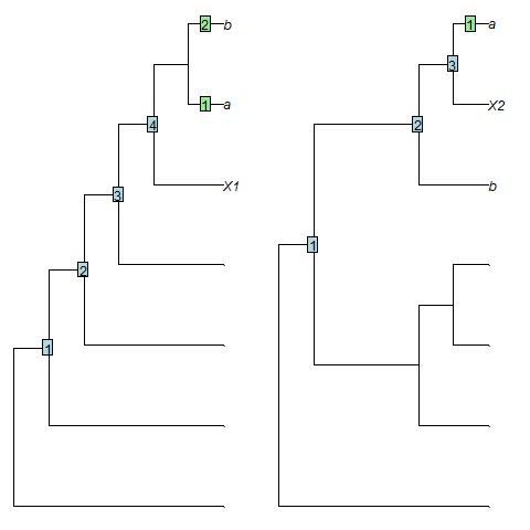
SisterSize() measures the number of leaves in the clade that is sister to
the chosen leaf, as proposed by Asher and Smith (2022).
In the examples above, X1 has a sister size of 2 leaves, whereas X2,
which is "more crownwards", has a smaller sister size (1 leaf), as desired.
Value
SisterSize() returns an integer specifying the number of leaves
in the clade that is sister to tip.
RootNodeDist() returns an integer specifying the number of nodes between
tip and the root node of tree.
Author(s)
Martin R. Smith (martin.smith@durham.ac.uk)
References
Asher R, Smith MR (2022). “Phylogenetic signal and bias in paleontology.” Systematic Biology, 71(4), 986–1008. doi:10.1093/sysbio/syab072.
See Also
Other tree characterization functions:
CladisticInfo(),
Consensus(),
J1Index(),
TotalCopheneticIndex()
Examples
bal8 <- BalancedTree(8)
pec8 <- PectinateTree(8)

SisterSize(bal8, 3)
SisterSize(pec8, "t3")
SisterSize(RootTree(pec8, "t3"), "t3")

RootNodeDist(bal8, 3)
RootNodeDist(pec8, "t3")
RootNodeDist(RootTree(pec8, "t3"), "t3")
Convert between strings and phyDat objects
Description
PhyDatToString() converts a phyDat object as a string;
StringToPhyDat() converts a string of character data to a phyDat object.
Usage
StringToPhyDat(string, tips, byTaxon = TRUE)

StringToPhydat(string, tips, byTaxon = TRUE)

PhyToString(
  phy,
  parentheses = "{",
  collapse = "",
  ps = "",
  useIndex = TRUE,
  byTaxon = TRUE,
  concatenate = TRUE
)

PhyDatToString(
  phy,
  parentheses = "{",
  collapse = "",
  ps = "",
  useIndex = TRUE,
  byTaxon = TRUE,
  concatenate = TRUE
)

PhydatToString(
  phy,
  parentheses = "{",
  collapse = "",
  ps = "",
  useIndex = TRUE,
  byTaxon = TRUE,
  concatenate = TRUE
)
Arguments
string |
String of tokens, optionally containing whitespace, with no terminating semi-colon. |
tips |
(Optional) Character vector corresponding to the names (in order) of each taxon in the matrix, or an object such as a tree from which tip labels can be extracted. |
byTaxon |
Logical. If |
phy |
An object of class |
parentheses |
Character specifying format of parentheses with which to
surround ambiguous tokens. Choose from: |
collapse |
Character specifying text, perhaps |
ps |
Character specifying text, perhaps |
useIndex |
Logical (default: |
concatenate |
Logical specifying whether to concatenate all characters/taxa into a single string, or to return a separate string for each entry. |
Value
StringToPhyDat() returns an object of class phyDat.
PhyToString() returns a character vector listing a text
representation of the phylogenetic character state for each taxon in turn.
Author(s)
Martin R. Smith (martin.smith@durham.ac.uk)
See Also
Other phylogenetic matrix conversion functions:
Decompose(),
MatrixToPhyDat(),
NexusTokensToInteger(),
Reweight()
Examples
StringToPhyDat("-?01231230?-", c("Lion", "Gazelle"), byTaxon = TRUE)
# encodes the following matrix:
# Lion     -?0123
# Gazelle  1230?-

fileName <- paste0(system.file(package = "TreeTools"),
                   "/extdata/input/dataset.nex")
phyDat <- ReadAsPhyDat(fileName)
PhyToString(phyDat, concatenate = FALSE)
Subset of a split on fewer leaves
Description
Subsplit() removes leaves from a Splits object.
Usage
Subsplit(splits, tips, keepAll = FALSE, unique = TRUE)
Arguments
splits |
An object of class |
tips |
A vector specifying a subset of the leaf labels applied to |
keepAll |
logical specifying whether to keep entries that define trivial splits (i.e. splits of zero or one leaf) on the subset of leaves. |
unique |
logical specifying whether to remove duplicate splits. |
Value
Subsplit() returns an object of class Splits, defined on the
leaves tips.
Author(s)
Martin R. Smith (martin.smith@durham.ac.uk)
See Also
KeepTip() is a less flexible but faster equivalent.
Other split manipulation functions:
DropTip(),
SplitConsistent(),
TrivialSplits()
Examples
splits <- as.Splits(PectinateTree(letters[1:9]))
splits
efgh <- Subsplit(splits, tips = letters[5:8], keepAll = TRUE)
summary(efgh)

TrivialSplits(efgh)

summary(Subsplit(splits, tips = letters[5:8], keepAll = FALSE))
Extract a subtree
Description
Subtree() safely extracts a clade from a phylogenetic tree.
Usage
Subtree(tree, node)
Arguments
tree |
A tree of class |
node |
The number of the node at the base of the clade to be extracted. |
Details
Modified from the ape function extract.clade, which
sometimes behaves unpredictably.
Unlike extract.clade, this function supports the extraction of "clades"
that constitute a single tip.
Value
Subtree() returns a tree of class phylo that represents a
clade extracted from the original tree.
Author(s)
Martin R. Smith (martin.smith@durham.ac.uk)
See Also
Other tree manipulation:
AddTip(),
CollapseNode(),
ConsensusWithout(),
DropTip(),
ImposeConstraint(),
KeptPaths(),
KeptVerts(),
LeafLabelInterchange(),
MakeTreeBinary(),
Renumber(),
RenumberTips(),
RenumberTree(),
RootTree(),
SortTree(),
TipTimedTree(),
TrivialTree
Examples
tree <- Preorder(BalancedTree(8))
plot(tree)
ape::nodelabels()
ape::nodelabels(13, 13, bg="yellow")

plot(Subtree(tree, 13))
Colour for node support value
Description
Colour value with which to display node support.
Usage
SupportColour(
  support,
  show1 = TRUE,
  scale = colorRampPalette(c("#D33F6A", "#e2e2e2", "#4A6FE3"))(101),
  outOfRange = "red"
)

SupportColor(
  support,
  show1 = TRUE,
  scale = colorRampPalette(c("#D33F6A", "#e2e2e2", "#4A6FE3"))(101),
  outOfRange = "red"
)
Arguments
support |
A numeric vector of values in the range 0–1. |
show1 |
Logical specifying whether to display values of 1.
A transparent white will be returned if |
scale |
101-element vector listing colours in sequence. Defaults to a diverging HCL scale. |
outOfRange |
Colour to use if results are outside the range 0–1. |
Value
SupportColour() returns the appropriate value from scale,
or outOfRange if a value is outwith the valid range.
See Also
Use in conjunction with LabelSplits() to colour split labels,
possibly calculated using SplitFrequency().
Examples
SupportColour((-1):4 / 4, show1 = FALSE)

# An example forest of 100 trees, some identical
forest <- as.phylo(c(1, rep(10, 79), rep(100, 15), rep(1000, 5)), nTip = 9)

# Generate an 80% consensus tree
cons <- ape::consensus(forest, p = 0.8)
plot(cons)

# Calculate split frequencies
splitFreqs <- SplitFrequency(cons, forest)

# Optionally, colour edges by corresponding frequency.
# Note that not all edges are associated with a unique split
# (and two root edges may be associated with one split - not handled here)
edgeSupport <- rep(1, nrow(cons$edge)) # Initialize trivial splits to 1
childNode <- cons$edge[, 2]
edgeSupport[match(names(splitFreqs), childNode)] <- splitFreqs / 100

plot(cons, edge.col = SupportColour(edgeSupport), edge.width = 3)

# Annotate nodes by frequency
LabelSplits(cons, splitFreqs, unit = "%",
            col = SupportColor(splitFreqs / 100),
            frame = "none", pos = 3L)
Extract tip labels
Description
TipLabels() extracts labels from an object: for example, names of taxa in
a phylogenetic tree or data matrix. AllTipLabels() extracts all labels,
where entries of a list of trees may pertain to different taxa.
Usage
TipLabels(x, single = TRUE)

## Default S3 method:
TipLabels(x, single = TRUE)

## S3 method for class 'matrix'
TipLabels(x, single = TRUE)

## S3 method for class 'logical'
TipLabels(x, single = TRUE)

## S3 method for class 'phylo'
TipLabels(x, single = TRUE)

## S3 method for class 'phyDat'
TipLabels(x, single = TRUE)

## S3 method for class 'MixedBase'
TipLabels(x, single = TRUE)

## S3 method for class 'TreeNumber'
TipLabels(x, single = TRUE)

## S3 method for class 'Splits'
TipLabels(x, single = TRUE)

## S3 method for class 'list'
TipLabels(x, single = FALSE)

## S3 method for class 'multiPhylo'
TipLabels(x, single = FALSE)

## S3 method for class 'character'
TipLabels(x, single = TRUE)

## S3 method for class 'numeric'
TipLabels(x, single = TRUE)

## S3 method for class 'phyDat'
TipLabels(x, single = TRUE)

AllTipLabels(x)

## S3 method for class 'list'
AllTipLabels(x)

## S3 method for class 'multiPhylo'
AllTipLabels(x)

## S3 method for class 'phylo'
AllTipLabels(x)

## S3 method for class 'Splits'
AllTipLabels(x)

## S3 method for class 'TreeNumber'
AllTipLabels(x)

## S3 method for class 'matrix'
AllTipLabels(x)
Arguments
x |
An object of a supported class (see Usage section above). |
single |
Logical specifying whether to report the labels for the first
object only ( |
Value
TipLabels() returns a character vector listing the tip labels
appropriate to x. If x is a single integer, this will be a vector
t1, t2 ... tx, to match the default of rtree().
Author(s)
Martin R. Smith (martin.smith@durham.ac.uk)
See Also
Other tree properties:
Cherries(),
ConsensusWithout(),
EdgeRatio(),
LongBranch(),
MatchEdges(),
NSplits(),
NTip(),
NodeNumbers(),
PathLengths(),
SplitsInBinaryTree(),
TreeIsRooted(),
Treeness()
Other Splits operations:
LabelSplits(),
NSplits(),
NTip(),
PolarizeSplits(),
SplitFrequency(),
Splits,
SplitsInBinaryTree(),
TipsInSplits(),
match,Splits,Splits-method,
xor()
Examples
TipLabels(BalancedTree(letters[5:1]))
TipLabels(5)

data("Lobo")
head(TipLabels(Lobo.phy))

AllTipLabels(c(BalancedTree(4), PectinateTree(8)))
Display time-calibrated tree using tip information only
Description
TipTimedTree() plots a phylogenetic tree against time using an
ad hoc approach based on dates associated with the leaves.
Nodes are dated to the youngest possible value, plus an additional "buffer"
(specified with minEdge) to ensure that branching order is readable.
Usage
TipTimedTree(tree, tipAge, minEdge = 1)
Arguments
tree |
A tree of class |
tipAge |
Numeric vector specifying the age (in units-of-time ago)
associated with each tip in |
minEdge |
Minimum length of edge to allow (in units-of-time) |
Details
This experimental function is liable to change its behaviour, or to be deprecated, in coming releases. Please contact the maintainer if you find it useful, so that a production-ready version can be prioritized.
Value
TipTimedTree() returns a tree with edge lengths set based on the
ages of each tip.
See Also
Other utility functions:
ClusterTable,
ClusterTable-methods,
Hamming(),
MSTEdges(),
SampleOne(),
UnshiftTree(),
as.multiPhylo(),
match,phylo,phylo-method,
sapply64(),
sort.multiPhylo()
Other tree manipulation:
AddTip(),
CollapseNode(),
ConsensusWithout(),
DropTip(),
ImposeConstraint(),
KeptPaths(),
KeptVerts(),
LeafLabelInterchange(),
MakeTreeBinary(),
Renumber(),
RenumberTips(),
RenumberTree(),
RootTree(),
SortTree(),
Subtree(),
TrivialTree
Examples
tree <- BalancedTree(6)
plot(TipTimedTree(tree, tipAge = 1:6, minEdge = 2))
Tips contained within splits
Description
TipsInSplits() specifies the number of tips that occur within each
bipartition split in a Splits object.
Usage
TipsInSplits(splits, keep.names = TRUE, smallest = FALSE, ...)

## S3 method for class 'Splits'
TipsInSplits(splits, keep.names = TRUE, smallest = FALSE, ...)

## S3 method for class 'phylo'
TipsInSplits(splits, keep.names = TRUE, smallest = FALSE, ...)

SplitImbalance(splits, keep.names = TRUE, ...)

## S3 method for class 'Splits'
SplitImbalance(splits, keep.names = TRUE, ...)

## S3 method for class 'phylo'
SplitImbalance(splits, keep.names = TRUE, ...)
Arguments
splits |
Object of class |
keep.names |
Logical specifying whether to include the names of |
smallest |
Logical; if |
... |
Additional parameters to pass to |
Value
TipsInSplits() returns a named vector of integers, specifying the
number of tips contained within each split in splits.
SplitImbalance() returns a named vector of integers, specifying the
number of leaves within a split that are not "balanced" by a leaf outside it;
i.e. a split that divides leaves evenly has an imbalance of zero; one that
splits two tips from ten has an imbalance of 10 - 2 = 8.
See Also
Other Splits operations:
LabelSplits(),
NSplits(),
NTip(),
PolarizeSplits(),
SplitFrequency(),
Splits,
SplitsInBinaryTree(),
TipLabels(),
match,Splits,Splits-method,
xor()
Examples
tree <- PectinateTree(8)
splits <- as.Splits(tree)
TipsInSplits(splits)

plot(tree)
LabelSplits(tree, as.character(splits), frame = "none", pos = 3L, cex = 0.7)
LabelSplits(tree, TipsInSplits(splits), unit = " tips", frame = "none",
            pos = 1L)
Remove metadata from trees
Description
TopologyOnly() removes all information from trees except for their
topologies and leaf labels.
Usage
TopologyOnly(tree)
Arguments
tree |
A tree of class |
Value
Returns tree, with each tree in Preorder, with edge lengths,
node labels and other attributes removed.
Author(s)
Martin R. Smith (martin.smith@durham.ac.uk)
Total Cophenetic Index
Description
TotalCopheneticIndex() calculates the total cophenetic index
(Mir et al. 2013) for any tree, a measure of its balance;
TCIContext() lists its possible values.
Usage
TotalCopheneticIndex(x)

TCIContext(x)

## S3 method for class 'numeric'
TCIContext(x)
Arguments
x |
A tree of class |
Details
The Total Cophenetic Index is a measure of tree balance – i.e. whether a (phylogenetic) tree comprises symmetric pairs of nodes, or has a pectinate "caterpillar" shape. The index has a greater resolution power than Sackin's and Colless' indices, and can be applied to trees that are not perfectly resolved.
For a tree with n leaves, the Total Cophenetic Index can take values of
0 to choose(n, 3).
The minimum value is higher for a perfectly resolved (i.e. dichotomous) tree
(see Lemma 14 of Mir et al. 2013).
Formulae to calculate the expected values under the Yule and Uniform models
of evolution are given in Theorems 17 and 23.
Full details are provided by Mir et al. (2013).
The J1 index
(Lemant et al. 2022) has advantages over the Total Cophenetic
Index, particularly when comparing trees with different numbers of leaves,
or where the population size of nodes is meaningful; see J1Index().
Value
TotalCopheneticIndex() returns an integer denoting the total cophenetic index.
TCIContext() returns a data frame detailing the maximum and minimum value
obtainable for the Total Cophenetic Index for rooted binary trees with the
number of leaves of the given tree, and the expected value under the Yule
and Uniform models.
The variance of the expected value is given under the Yule model, but cannot
be obtained by calculation for the Uniform model.
Author(s)
Martin R. Smith (martin.smith@durham.ac.uk)
References
Lemant J, Le Sueur C, Manojlović V, Noble R (2022).
“Robust, Universal Tree Balance Indices.”
Systematic Biology, 71(5), 1210–1224.
doi:10.1093/sysbio/syac027.
Mir A, Rosselló F, Rotger LA (2013).
“A new balance index for phylogenetic trees.”
Mathematical Biosciences, 241(1), 125–136.
doi:10.1016/j.mbs.2012.10.005.
See Also
-
J1Index()provides a more robust, universal tree balance index. -
cophen.index()in the package CollessLike provides an alternative implementation of this index and its predecessors.
Other tree characterization functions:
CladisticInfo(),
Consensus(),
J1Index(),
Stemwardness
Examples
# Balanced trees have the minimum index for a binary tree;
# Pectinate trees the maximum:
TCIContext(8)
TotalCopheneticIndex(PectinateTree(8))
TotalCopheneticIndex(BalancedTree(8))
TotalCopheneticIndex(StarTree(8))


# Examples from Mir et al. (2013):
tree12 <- ape::read.tree(text="(1, (2, (3, (4, 5))));")  #Fig. 4, tree 12
TotalCopheneticIndex(tree12) # 10
tree8  <- ape::read.tree(text="((1, 2, 3, 4), 5);")      #Fig. 4, tree 8
TotalCopheneticIndex(tree8)  # 6
TCIContext(tree8)
TCIContext(5L) # Context for a tree with 5 leaves.
Is tree rooted?
Description
TreeIsRooted() is a fast alternative to ape::is.rooted().
Usage
TreeIsRooted(tree)
Arguments
tree |
A phylogenetic tree of class |
Value
TreeIsRooted() returns a logical specifying whether a root node is
resolved.
Author(s)
Martin R. Smith (martin.smith@durham.ac.uk)
See Also
Other tree properties:
Cherries(),
ConsensusWithout(),
EdgeRatio(),
LongBranch(),
MatchEdges(),
NSplits(),
NTip(),
NodeNumbers(),
PathLengths(),
SplitsInBinaryTree(),
TipLabels(),
Treeness()
Examples
TreeIsRooted(BalancedTree(6))
TreeIsRooted(UnrootTree(BalancedTree(6)))
Unique integer indices for bifurcating tree topologies
Description
Functions converting between phylogenetic trees and their unique decimal representation, based on a concept by John Tromp, employed in Li et al. (1996).
Usage
as.TreeNumber(x, ...)

## S3 method for class 'phylo'
as.TreeNumber(x, ...)

## S3 method for class 'multiPhylo'
as.TreeNumber(x, ...)

## S3 method for class 'character'
as.TreeNumber(x, nTip, tipLabels = TipLabels(nTip), ...)

## S3 method for class 'TreeNumber'
as.TreeNumber(x, ...)

## S3 method for class 'MixedBase'
as.TreeNumber(x, ...)

## S3 method for class 'TreeNumber'
as.MixedBase(x, ...)

## S3 method for class 'integer64'
as.MixedBase(x, tipLabels = NULL, ...)

## S3 method for class 'numeric'
as.MixedBase(x, tipLabels = NULL, ...)

## S3 method for class 'numeric'
as.phylo(x, nTip = attr(x, "nTip"), tipLabels = attr(x, "tip.label"), ...)

## S3 method for class 'TreeNumber'
as.phylo(x, nTip = attr(x, "nTip"), tipLabels = attr(x, "tip.label"), ...)

as.MixedBase(x, ...)

## S3 method for class 'MixedBase'
as.MixedBase(x, ...)

## S3 method for class 'phylo'
as.MixedBase(x, ...)

## S3 method for class 'multiPhylo'
as.MixedBase(x, ...)

## S3 method for class 'MixedBase'
as.phylo(x, nTip = attr(x, "nTip"), tipLabels = attr(x, "tip.label"), ...)
Arguments
x |
Integer identifying the tree (see details). |
... |
Additional parameters for consistency with S3 methods (unused). |
nTip |
Integer specifying number of leaves in the tree. |
tipLabels |
Character vector listing the labels assigned to each tip
in a tree, perhaps obtained using |
Details
There are NUnrooted(n) unrooted trees with n leaves.
As such, each n-leaf tree can be uniquely identified by a non-negative
integer x < NUnrooted(n).
This integer can be converted by a tree by treating it as a mixed-base number, with bases 1, 3, 5, 7, … (2 n - 5).
Each digit of this mixed base number corresponds to a leaf, and determines the location on a growing tree to which that leaf should be added.
We start with a two-leaf tree, and treat 0 as the origin of the tree.
0 ---- 1
We add leaf 2 by breaking an edge and inserting a node (numbered
2 + nTip - 1).
In this example, we'll work up to a six-leaf tree; this node will be numbered
2 + 6 - 1 = 7.
There is only one edge on which leaf 2 can be added. Let's add node 7 and
leaf 2:
0 ---- 7 ---- 1
       |
       |
       2
There are now three edges on which leaf 3 can be added. Our options are:
Option 0: the edge leading to 1;
Option 1: the edge leading to 2;
Option 2: the edge leading to 7.
If we select option 1, we produce:
0 ---- 7 ---- 1
       |
       |
       8 ---- 2
       |
       |
       3
1 is now the final digit of our mixed-base number.
There are five places to add leaf 4:
Option 0: the edge leading to 1;
Option 1: the edge leading to 2;
Option 2: the edge leading to 3;
Option 3: the edge leading to 7;
Option 4: the edge leading to 8.
If we chose option 3, then 3 would be the penultimate digit of our
mixed-base number.
If we chose option 0 for the next two additions, we could specify this tree with the mixed-base number 0021. We can convert this into decimal:
0 × (1 × 3 × 5 × 9) +
0 × (1 × 3 × 5) +
3 × (1 × 3) +
1 × (1)
= 10
as.TreeNumber() supports up to 51 leaves.
For trees with at most 19 leaves, the number fits in a 64-bit integer and
the TreeNumber is stored as an integer64 (via the bit64 package),
enabling arithmetic and exact round-tripping via as.MixedBase().
For trees with 20–51 leaves, there are more than 2^64 distinct topologies,
so the tree number is stored as a decimal character string instead.
Package developers can use the C++ header TreeTools/tree_number.h
(via LinkingTo: TreeTools) for the underlying 256-bit encoding
(tree_num_t) directly.
Value
as.TreeNumber() returns an object of class TreeNumber with
attributes nTip and tip.label.
For trees with at most 19 leaves the underlying storage is a single
integer64 value (class c("TreeNumber", "integer64")), enabling
integer64 arithmetic and exact round-tripping through as.MixedBase().
For trees with 20–51 leaves the number exceeds 2^64, so it is stored as a
decimal character string (class c("TreeNumber", "character")).
If x is a list of trees or a multiPhylo object,
as.TreeNumber() returns a corresponding list of TreeNumber objects.
as.phylo.numeric() returns a tree of class phylo.
Author(s)
Martin R. Smith (martin.smith@durham.ac.uk)
References
Li M, Tromp J, Zhang L (1996). “Some notes on the nearest neighbour interchange distance.” In Goos G, Hartmanis J, Leeuwen J, Cai J, Wong CK (eds.), Computing and Combinatorics, volume 1090, 343–351. Springer, Berlin, Heidelberg. ISBN 978-3-540-61332-9. doi:10.1007/3-540-61332-3_168.
See Also
Describe the shape of a tree topology, independent of leaf labels:
TreeShape()
Other tree generation functions:
ConstrainedNJ(),
GenerateTree,
NJTree(),
TrivialTree
Other 'TreeNumber' utilities:
is.TreeNumber(),
print.TreeNumber()
Examples
tree <- as.phylo(10, nTip = 6)
plot(tree)
as.TreeNumber(tree)

# Trees with 20--51 leaves are stored as decimal strings:
as.TreeNumber(BalancedTree(19))  # integer64-backed
as.TreeNumber(BalancedTree(51))  # character-backed

# If > 9 digits, represent the tree number as a string.
treeNumber <- as.TreeNumber("1234567890123", nTip = 14)
tree <- as.phylo(treeNumber)
as.phylo(0:2, nTip = 6, tipLabels = letters[1:6])
Relative length of internal branches
Description
Treeness (also termed stemminess) is the proportion of a tree's length found on internal branches (Lanyon 1988). Insofar as external branches do not contain phylogenetic (grouping) signal, trees with a high treeness can be interpreted as containing a higher signal:noise ratio (Phillips and Penny 2003-08).
Usage
Treeness(tree)

Stemminess(tree)
Arguments
tree |
A tree of class |
Value
Treeness() returns a numeric vector reporting the treeness of each
tree.
Author(s)
Martin R. Smith (martin.smith@durham.ac.uk)
References
Lanyon SM (1988).
“The Stochastic Mode of Molecular Evolution: What Consequences for Systematic Investigations?”
The Auk, 105(3), 565–573.
doi:10.1093/auk/105.3.565.
Phillips MJ, Penny D (2003-08).
“The Root of the Mammalian Tree Inferred from Whole Mitochondrial Genomes.”
Molecular Phylogenetics and Evolution, 28(2), 171–185.
doi:10.1016/S1055-7903(03)00057-5.
See Also
Other tree properties:
Cherries(),
ConsensusWithout(),
EdgeRatio(),
LongBranch(),
MatchEdges(),
NSplits(),
NTip(),
NodeNumbers(),
PathLengths(),
SplitsInBinaryTree(),
TipLabels(),
TreeIsRooted()
Examples
lowTree <- BalancedTree(6, lengths = c(1, 1, 4, 4, 4, 1, 1, 4, 4, 4))
plot(lowTree)
Treeness(lowTree)
highTree <- BalancedTree(6, lengths = c(6, 6, 1, 1, 1, 6, 6, 1, 1, 1))
plot(highTree)
Treeness(c(lowTree, highTree))
Number of trees matching a bipartition split
Description
Calculates the number of unrooted bifurcated trees that are consistent with
a bipartition split that divides taxa into groups of size A and B.
Usage
TreesMatchingSplit(A, B = A[2])

LnTreesMatchingSplit(A, B = A[2])

Log2TreesMatchingSplit(A, B = A[2])
Arguments
A, B |
Integer specifying the number of taxa in each partition. |
Value
TreesMatchingSplit() returns a numeric specifying the number of trees
that are compatible with the given split.
LnTreesMatchingSplit() and Log2TreesMatchingSplit() give the natural
and base-2 logarithms of this number.
Author(s)
Martin R. Smith (martin.smith@durham.ac.uk)
See Also
Other split information functions:
CharacterInformation(),
SplitInformation(),
SplitMatchProbability(),
UnrootedTreesMatchingSplit()
Examples
TreesMatchingSplit(5, 6)
LnTreesMatchingSplit(5, 6)
Log2TreesMatchingSplit(5, 6)
Number of trees containing a tree
Description
TreesMatchingTree() calculates the number of unrooted binary trees that
are consistent with a tree topology on the same leaves.
Usage
TreesMatchingTree(tree)

LnTreesMatchingTree(tree)

Log2TreesMatchingTree(tree)
Arguments
tree |
A tree of class |
Details
Remember to unroot a tree first if the position of its root is arbitrary.
Value
TreesMatchingTree() returns a numeric specifying the number of
unrooted binary trees that contain all the edges present in the input tree.
LnTreesMatchingTree() gives the natural logarithm of this number.
Author(s)
Martin R. Smith (martin.smith@durham.ac.uk)
See Also
Other tree information functions:
CladisticInfo(),
NRooted()
Examples
partiallyResolvedTree <- CollapseNode(BalancedTree(8), 12:15)
TreesMatchingTree(partiallyResolvedTree)
LnTreesMatchingTree(partiallyResolvedTree)

# Number of rooted trees:
rootedTree <- AddTip(partiallyResolvedTree, where = 0)
TreesMatchingTree(partiallyResolvedTree)
Identify and remove trivial splits
Description
TrivialSplits() identifies trivial splits (which separate one or zero
leaves from all others); WithoutTrivialSplits() removes them from a
Splits object.
Usage
TrivialSplits(splits, nTip = attr(splits, "nTip"))

WithoutTrivialSplits(splits, nTip = attr(splits, "nTip"))
Arguments
splits |
An object of class |
nTip |
Integer specifying number of tips (leaves). |
Value
TrivialSplits() returns a logical vector specifying whether each
split in splits is trivial, i.e. includes or excludes only a single tip or
no tips at all.
WithoutTrivialSplits() returns a Splits object with trivial
splits removed.
Author(s)
Martin R. Smith (martin.smith@durham.ac.uk)
See Also
Other split manipulation functions:
DropTip(),
SplitConsistent(),
Subsplit()
Examples
splits <- as.Splits(PectinateTree(letters[1:9]))
efgh <- Subsplit(splits, tips = letters[5:8], keepAll = TRUE)
summary(efgh)

TrivialSplits(efgh)
summary(WithoutTrivialSplits(efgh))
Generate trivial trees
Description
SingleTaxonTree() creates a phylogenetic "tree" that contains a single
taxon.
ZeroTaxonTree() creates an empty phylo object with zero leaves or edges.
Usage
SingleTaxonTree(label = "t1", lengths = NULL)

ZeroTaxonTree()
Arguments
label |
a character vector specifying the label of the tip. |
lengths |
Numeric vector of edge lengths, or a function that returns
such a vector when passed the number of edges as its argument (e.g. |
Value
SingleTaxonTree() returns a phylo object containing a single
tip with the specified label.
ZeroTaxonTree() returns an empty phylo object.
See Also
Other tree manipulation:
AddTip(),
CollapseNode(),
ConsensusWithout(),
DropTip(),
ImposeConstraint(),
KeptPaths(),
KeptVerts(),
LeafLabelInterchange(),
MakeTreeBinary(),
Renumber(),
RenumberTips(),
RenumberTree(),
RootTree(),
SortTree(),
Subtree(),
TipTimedTree()
Other tree generation functions:
ConstrainedNJ(),
GenerateTree,
NJTree(),
TreeNumber
Examples
SingleTaxonTree("Homo_sapiens")
plot(SingleTaxonTree("root") + BalancedTree(4))

ZeroTaxonTree()
Remove quotation marks from a string
Description
Remove quotation marks from a string
Usage
Unquote(string)
Arguments
string |
Input string |
Value
Unquote() returns string, with any matched punctuation marks
and trailing whitespace removed.
Author(s)
Martin R. Smith
See Also
Other string parsing functions:
EndSentence(),
MatchStrings(),
MorphoBankDecode(),
RightmostCharacter()
Examples
Unquote("'Hello World'")
Number of trees consistent with split
Description
Calculates the number of unrooted bifurcating trees consistent with the specified multi-partition split, using theorem two of Carter et al. (1990).
Usage
UnrootedTreesMatchingSplit(...)

LnUnrootedTreesMatchingSplit(...)

Log2UnrootedTreesMatchingSplit(...)
Arguments
... |
A series or vector of integers listing the number of tips in
each of a number of tree splits (e.g. bipartitions).
For example, |
Value
UnrootedTreesMatchingSplit() returns an integer specifying the
number of unrooted bifurcating trees consistent with the specified split.
Author(s)
Martin R. Smith (martin.smith@durham.ac.uk)
References
Carter M, Hendy M, Penny D, Székely LA, Wormald NC (1990). “On the distribution of lengths of evolutionary trees.” SIAM Journal on Discrete Mathematics, 3(1), 38–47. doi:10.1137/0403005.
See Also
Other split information functions:
CharacterInformation(),
SplitInformation(),
SplitMatchProbability(),
TreesMatchingSplit()
Examples
UnrootedTreesMatchingSplit(c(3, 5))
UnrootedTreesMatchingSplit(3, 2, 1, 2)
Add tree to start of list
Description
UnshiftTree() adds a phylogenetic tree to the start of a list of trees.
This is useful where the class of a list of trees is unknown, or where
names of trees should be retained.
Usage
UnshiftTree(add, treeList)
Arguments
add |
Tree to add to the list, of class |
treeList |
A list of trees, of class |
Details
Caution: adding a tree to a multiPhylo object whose own attributes apply
to all trees, for example trees read from a Nexus file, causes data to be
lost.
Value
UnshiftTree() returns a list of class list or multiPhylo
(following the original class of treeList), whose first element is the
tree specified as 'add.
Author(s)
Martin R. Smith (martin.smith@durham.ac.uk)
See Also
c() joins a tree or series of trees to a multiPhylo object, but loses
names and does not handle lists of trees.
Other utility functions:
ClusterTable,
ClusterTable-methods,
Hamming(),
MSTEdges(),
SampleOne(),
TipTimedTree(),
as.multiPhylo(),
match,phylo,phylo-method,
sapply64(),
sort.multiPhylo()
Examples
forest <- as.phylo(0:5, 6)
tree <- BalancedTree(6)

UnshiftTree(tree, forest)
UnshiftTree(tree, tree)
Write morphological character matrix to TNT file
Description
Write morphological character matrix to TNT file
Usage
WriteTntCharacters(
  dataset,
  filepath = NULL,
  comment = "Dataset written by `TreeTools::WriteTntCharacters()`",
  types = NULL,
  pre = "",
  post = ""
)

## S3 method for class 'phyDat'
WriteTntCharacters(
  dataset,
  filepath = NULL,
  comment = "Dataset written by `TreeTools::WriteTntCharacters()`",
  types = NULL,
  pre = "",
  post = ""
)

## S3 method for class 'matrix'
WriteTntCharacters(
  dataset,
  filepath = NULL,
  comment = "Dataset written by `TreeTools::WriteTntCharacters()`",
  types = NULL,
  pre = "",
  post = ""
)
Arguments
dataset |
Morphological dataset of class |
filepath |
Path to file; if |
comment |
Optional comment with which to entitle matrix. |
types |
Optional list specifying where different data types begin.
|
pre, post |
Character vector listing text to print before and after the
character matrix. Specify |
Author(s)
Martin R. Smith (martin.smith@durham.ac.uk)
See Also
Examples
data("Lobo", package = "TreeTools")

WriteTntCharacters(Lobo.phy)

# Read with extended implied weighting
WriteTntCharacters(Lobo.phy, pre = "piwe=10;", post = "xpiwe=;")

# Write to a file with:
# WriteTntCharacters(Lobo.phy, "example_file.tnt")
Write a phylogenetic tree in Newick format
Description
as.Newick() creates a character string representation of a phylogenetic
tree, in the Newick format, using R's internal tip numbering.
Use RenumberTips() to ensure that the internal numbering follows the
order you expect.
Usage
as.Newick(x)

## S3 method for class 'phylo'
as.Newick(x)

## S3 method for class 'list'
as.Newick(x)

## S3 method for class 'multiPhylo'
as.Newick(x)
Arguments
x |
Object to convert to Newick format. See Usage section for supported classes. |
Value
as.Newick() returns a character string representing tree in Newick
format.
Author(s)
Martin R. Smith (martin.smith@durham.ac.uk)
See Also
Retain leaf labels:
NewickTree()Change R's internal numbering of leaves:
RenumberTips()Write tree to text or file:
ape::write.tree()
Examples
trees <- list(BalancedTree(1:8), PectinateTree(8:1))
trees <- lapply(trees, RenumberTips, 1:8)
as.Newick(trees)
Convert object to multiPhylo class
Description
Converts representations of phylogenetic trees to an object of the "ape"
class multiPhylo.
Usage
as.multiPhylo(x)

## S3 method for class 'phylo'
as.multiPhylo(x)

## S3 method for class 'list'
as.multiPhylo(x)

## S3 method for class 'phyDat'
as.multiPhylo(x)

## S3 method for class 'Splits'
as.multiPhylo(x)
Arguments
x |
Object to be converted |
Value
as.multiPhylo returns an object of class multiPhylo
as.multiPhylo.phyDat() returns a list of trees, each corresponding
to the partitions implied by each non-ambiguous character in x.
See Also
Other utility functions:
ClusterTable,
ClusterTable-methods,
Hamming(),
MSTEdges(),
SampleOne(),
TipTimedTree(),
UnshiftTree(),
match,phylo,phylo-method,
sapply64(),
sort.multiPhylo()
Examples
as.multiPhylo(BalancedTree(8))
as.multiPhylo(list(BalancedTree(8), PectinateTree(8)))
data("Lobo")
as.multiPhylo(Lobo.phy)
Brewer palettes
Description
A list of eleven Brewer palettes containing one to eleven colours that are readily distinguished by colourblind viewers, followed by a twelfth 12-colour palette adapted for colour blindness.
Usage
brewer
Format
An object of class list of length 12.
Source
Examples
data("brewer", package = "TreeTools")
plot(0, type = "n", xlim = c(1, 12), ylim = c(12, 1),
     xlab = "Colour", ylab="Palette")
for (i in seq_along(brewer)) text(seq_len(i), i, col = brewer[[i]])
Double factorials
Description
A vector with pre-calculated values of double factorials up to 300!!, and the logarithms of double factorials up to 50 000!!.
Usage
doubleFactorials
Format
An object of class numeric of length 300.
Details
301!! is too large to store as an integer; use logDoubleFactorials instead.
See Also
Other double factorials:
DoubleFactorial(),
logDoubleFactorials
Efficiently convert edge matrix to splits
Description
Wrapper for internal C++ function for maximum efficiency. Improper input may crash R. Behaviour not guaranteed. It is advisable to contact the package maintainers before relying on this function.
Usage
edge_to_splits(
  edge,
  edgeOrder,
  tipLabels = NULL,
  asSplits = TRUE,
  nTip = NTip(edge),
  ...
)
Arguments
edge |
A matrix with two columns, with each row listing the parent and
child node of an edge in a phylogenetic tree. Property |
edgeOrder |
Integer vector such that |
tipLabels |
Character vector specifying sequence in which to order
tip labels. Label order must (currently) match to combine or compare separate
|
asSplits |
Logical specifying whether to return a |
nTip |
Integer specifying number of leaves in tree. |
... |
Presently unused. |
Value
edge_to_splits() uses the same return format as as.Splits().
See Also
as.Splits() offers a safe access point to this
function that should be suitable for most users.
Is an object a TreeNumber object?
Description
Is an object a TreeNumber object?
Usage
is.TreeNumber(x)
Arguments
x |
R object. |
Value
is.TreeNumber() returns a logical vector of length one specifying
whether x inherits the class "TreeNumber".
Author(s)
Martin R. Smith (martin.smith@durham.ac.uk)
See Also
Other 'TreeNumber' utilities:
TreeNumber,
print.TreeNumber()
Examples
is.TreeNumber(FALSE) # FALSE
is.TreeNumber(as.TreeNumber(BalancedTree(5))) # TRUE
Natural logarithms of double factorials
Description
logDoubleFactorials is a numeric vector with pre-calculated values of
double factorials up to 50 000!!.
Usage
logDoubleFactorials
Format
An object of class numeric of length 50000.
See Also
Other double factorials:
DoubleFactorial(),
doubleFactorials
Split matching
Description
match() returns a vector of the positions of (first) matches of splits in
its first argument in its second.
%in% is a more intuitive interface as a binary operator, which returns
a logical vector indicating whether there is a match or not for each
split in its left operand.
Usage
## S4 method for signature 'Splits,Splits'
match(x, table, nomatch = NA_integer_, incomparables = NULL)

match(x, table, nomatch = NA_integer_, incomparables = NULL)

## S4 method for signature 'Splits,Splits'
x %in% table

FirstMatchingSplit(x, table, nomatch, return = c("x", "table", "both"))
Arguments
x, table |
Splits objects |
nomatch |
Integer value that will be used in place of |
incomparables |
Ignored. (Included for consistency with generic.) |
return |
Which index to return: in |
Value
match() returns an integer vector specifying the position in
table that matches each element in x, or nomatch if no match is found.
FirstMatchingSplit() returns an integer
(or length-2 integer if return = "both") specifying the first split in x
to have a match in table (return = "x"),
or the index of that match (return = "table").
nomatch (default 0) is returned in the absence of a match.
See Also
Corresponding base functions are documented in
match().
Other Splits operations:
LabelSplits(),
NSplits(),
NTip(),
PolarizeSplits(),
SplitFrequency(),
Splits,
SplitsInBinaryTree(),
TipLabels(),
TipsInSplits(),
xor()
Examples
splits1 <- as.Splits(BalancedTree(7))
splits2 <- as.Splits(PectinateTree(7))

match(splits1, splits2)
Tree matching
Description
match() returns a vector of the positions of (first) matches of trees in
its first argument in its second.
%in% is a more intuitive interface as a binary operator, which returns
a logical vector indicating whether there is a match or not for each
tree in its left operand.
Usage
## S4 method for signature 'phylo,phylo'
match(x, table, nomatch = NA_integer_, incomparables = NULL)

## S4 method for signature 'multiPhylo,phylo'
match(x, table, nomatch = NA_integer_, incomparables = NULL)

## S4 method for signature 'phylo,multiPhylo'
match(x, table, nomatch = NA_integer_, incomparables = NULL)

## S4 method for signature 'multiPhylo,multiPhylo'
match(x, table, nomatch = NA_integer_, incomparables = NULL)

## S4 method for signature 'multiPhylo,multiPhylo'
x %in% table

## S4 method for signature 'multiPhylo,phylo'
x %in% table

## S4 method for signature 'phylo,multiPhylo'
x %in% table

## S4 method for signature 'phylo,phylo'
x %in% table
Arguments
x, table |
Object of class |
nomatch |
Integer value that will be used in place of |
incomparables |
Ignored. (Included for consistency with generic.) |
Value
match() returns an integer vector specifying the position in
table that matches each element in x, or nomatch if no match is found.
See Also
Corresponding base functions are documented in
match().
Other utility functions:
ClusterTable,
ClusterTable-methods,
Hamming(),
MSTEdges(),
SampleOne(),
TipTimedTree(),
UnshiftTree(),
as.multiPhylo(),
sapply64(),
sort.multiPhylo()
Examples
tree1 <- BalancedTree(7)
trees <- c(PectinateTree(7), BalancedTree(7))

match(tree1, trees)
Number of rooted / unrooted tree shapes
Description
nRootedShapes and nUnrootedShapes give the number of (un)rooted binary
trees on n unlabelled leaves.
Usage
nRootedShapes

nUnrootedShapes
Format
An object of class integer64 of length 55.
An object of class integer64 of length 60.
Source
nRootedShapes corresponds to the Wedderburn-Etherington numbers,
OEIS A001190
nUnrootedShapes is OEIS A000672
Print TreeNumber object
Description
S3 method for objects of class TreeNumber.
Usage
## S3 method for class 'TreeNumber'
print(x, ...)
Arguments
x |
Object of class |
... |
Additional arguments for consistency with S3 method (unused). |
See Also
Other 'TreeNumber' utilities:
TreeNumber,
is.TreeNumber()
Wrapper for internal C function root_on_node()
Description
Direct entry point to root_on_node(); recommended for expert use only.
RootTree() checks that input is properly formatted and is recommended
for general use.
Usage
root_on_node(phy, outgroup)
Arguments
phy |
Minimally, a named list with entries |
outgroup |
Integer specifying index of leaf or node to set as the outgroup. |
Value
root_on_node() returns phy rooted on the specified node.
Author(s)
Martin R. Smith (martin.smith@durham.ac.uk)
Apply a function that returns 64-bit integers over a list or vector
Description
Wrappers for members of the lapply() family intended for use when a
function FUN returns a vector of integer64 objects.
vapply(), sapply() or replicate() drop the integer64 class,
resulting in a vector of numerics that require conversion back to
64-bit integers. These functions restore the missing class attribute.
Usage
sapply64(X, FUN, ..., simplify = TRUE, USE.NAMES = TRUE)

vapply64(X, FUN, FUN.LEN = 1, ...)

replicate64(n, expr, simplify = "array")
Arguments
X |
a vector (atomic or list) or an |
FUN |
the function to be applied to each element of |
... |
optional arguments to |
simplify |
logical or character string; should the result be
simplified to a vector, matrix or higher dimensional array if
possible? For |
USE.NAMES |
logical; if |
FUN.LEN |
Integer specifying the length of the output of |
n |
integer: the number of replications. |
expr |
the expression (a language object, usually a call) to evaluate repeatedly. |
Details
For details of the underlying functions, see base::lapply().
Author(s)
Martin R. Smith (martin.smith@durham.ac.uk)
See Also
Other utility functions:
ClusterTable,
ClusterTable-methods,
Hamming(),
MSTEdges(),
SampleOne(),
TipTimedTree(),
UnshiftTree(),
as.multiPhylo(),
match,phylo,phylo-method,
sort.multiPhylo()
Examples
sapply64(as.phylo(1:6, 6), as.TreeNumber)
vapply64(as.phylo(1:6, 6), as.TreeNumber, 1)
set.seed(0)
replicate64(6, as.TreeNumber(RandomTree(6)))
Sort a list of phylogenetic trees
Description
Trees are sorted by their mixed base representation, treating their leaves in the order of their labels (i.e. alphabetically, if leaves are labelled with text).
Usage
## S3 method for class 'multiPhylo'
sort(x, decreasing = FALSE, na.last = NA, ...)

## S3 method for class 'phylo'
e1 == e2

## S3 method for class 'phylo'
e1 < e2

## S3 method for class 'phylo'
e1 > e2

## S3 method for class 'MixedBase'
e1 == e2

## S3 method for class 'MixedBase'
e1 < e2

## S3 method for class 'MixedBase'
e1 > e2
Arguments
x, decreasing, na.last, ... |
As in |
e1, e2 |
Objects to be compared. |
Author(s)
Martin R. Smith (martin.smith@durham.ac.uk)
See Also
Other utility functions:
ClusterTable,
ClusterTable-methods,
Hamming(),
MSTEdges(),
SampleOne(),
TipTimedTree(),
UnshiftTree(),
as.multiPhylo(),
match,phylo,phylo-method,
sapply64()
Examples
sort(as.phylo(5:0, 7))
Integer representing shape of a tree
Description
Returns an integer that uniquely represents the shape of an n-tip binary tree, ignoring tip labels.
Usage
unrootedKeys

RootedTreeShape(tree)

RootedTreeWithShape(shape, nTip, tipLabels)

UnrootedTreeWithShape(shape, nTip, tipLabels = character(nTip))

UnrootedTreeWithKey(key, nTip, tipLabels = character(nTip))

UnrootedTreeShape(tree)

UnrootedTreeKey(tree, asInteger = FALSE)

.UnrootedKeys(nTip)

UnrootedKeys(nTip, ...)

NUnrootedShapes(nTip)

NRootedShapes(nTip)
Arguments
tree |
A tree of class |
shape |
Integer specifying shape of tree, perhaps generated by
|
nTip |
Integer specifying number of tips. |
tipLabels |
Character vector listing the labels assigned to each tip
in a tree, perhaps obtained using |
key |
Integer specifying the key (not number) of an unrooted tree. |
asInteger |
Logical specifying whether to coerce the return value to
mode |
... |
Deprecated (2025-09); retained for backward compatibility. |
Format
unrootedKeys is a list of length 22; each
entry is a vector of integers corresponding to the keys (not shape numbers)
of the different unrooted tree shapes with nTip leaves.
Details
Rooted trees are numbered working up from the root.
The root node divides n tips into two subtrees. The smaller subtree may contain $a = 1, 2, ..., n/2$ tips, leaving $b = n - a$ tips in These options are worked through in turn.
For the first shape of the smaller subtree, work through each possible shape for the larger subtree. Then, move to the next shape of the smaller subtree, and work through each possible shape of the larger subtree.
Stop when the desired topology is encountered.
Unrooted trees are numbered less elegantly. Each cherry (i.e. node subtending a pair of tips) is treated in turn. The subtended tips are removed, and the node treated as the root of a rooted tree. The number of this rooted tree is then calculated. The tree is assigned a key corresponding to the lowest such value. The keys of all unrooted tree shapes on n tips are ranked, and the unrooted tree shape is assigned a number based on the rank order of its key among all possible keys, counting from zero.
If UnrootedTreeShape() or UnrootedTreeKey() is passed a rooted tree,
the position of the root will be ignored.
The number of unlabelled binary rooted trees corresponds to the Wedderburn-Etherington numbers.
Value
TreeShape() returns an integer specifying the shape of a tree,
ignoring tip labels.
RootedTreeWithShape() returns a tree of class phylo
corresponding to the shape provided. Tips are unlabelled.
UnrootedTreeWithShape() returns a tree of class phylo
corresponding to the shape provided. Tips are unlabelled.
UnrootedTreeWithKey() returns a tree of class phylo corresponding
to the key provided. Tips are unlabelled.
UnrootedKeys() returns a vector of integers corresponding to the
keys (not shape numbers) of unrooted tree shapes with nTip tips.
It is a wrapper to .UnrootedKeys(), with memoization, meaning that results
once calculated are cached and need not be calculated on future calls to
the function.
NUnrootedShapes() returns an object of class integer64 specifying
the number of unique unrooted tree shapes with nTip (< 61) tips.
NRootedShapes() returns an object of class integer64 specifying
the number of unique rooted tree shapes with nTip (< 56) leaves.
Author(s)
Martin R. Smith (martin.smith@durham.ac.uk)
See Also
Unique number for a labelled tree: TreeNumber()
Examples
RootedTreeShape(PectinateTree(8))
plot(RootedTreeWithShape(0, nTip = 8L))

NRootedShapes(8L)
# Shapes are numbered from 0 to NRootedShapes(n) - 1.  The maximum shape is:
RootedTreeShape(BalancedTree(8))

# Unique shapes of unrooted trees:
NUnrootedShapes(8L)

# Keys of these trees:
UnrootedKeys(8L)

# A tree may be represented by multiple keys.
# For a one-to-one correspondence, use a number instead:
unrootedShapes8 <- as.integer(NUnrootedShapes(8L))
allShapes <- lapply(seq_len(unrootedShapes8) - 1L,
                    UnrootedTreeWithShape, 8L)
plot(allShapes[[1]])
sapply(allShapes, UnrootedTreeShape)
sapply(allShapes, UnrootedTreeKey, asInteger = TRUE) # Key >= number

# If numbers larger than 2>31 are required, sapply needs a little help
# with 64-bit integers:
structure(sapply(allShapes, UnrootedTreeKey), class = "integer64")
Exclusive OR operation
Description
Exclusive OR operation
Usage
xor(x, y)

## S4 method for signature 'Splits,Splits'
xor(x, y)
Arguments
x, y |
Objects to be compared. |
See Also
Other Splits operations:
LabelSplits(),
NSplits(),
NTip(),
PolarizeSplits(),
SplitFrequency(),
Splits,
SplitsInBinaryTree(),
TipLabels(),
TipsInSplits(),
match,Splits,Splits-method