| Title: | SEER and Atomic Bomb Survivor Data Analysis Tools |
| Version: | 2019.2 |
| Date: | 2019-12-12 |
| Description: | Creates SEER (Surveillance, Epidemiology and End Results) and A-bomb data binaries from ASCII sources and provides tools for estimating SEER second cancer risks. Methods are described in <doi:10.1038/leu.2015.258>. |
| Depends: | dplyr, ggplot2, rgl, demography |
| Suggests: | bbmle |
| License: | GPL-2 | GPL-3 [expanded from: GPL (≥ 2)] |
| Imports: | Rcpp (≥ 0.11.3), reshape2, mgcv, tibble, LaF, DBI, RSQLite, openxlsx, WriteXLS, labelled, scales, forcats, purrr,readr, tidyr, stringr, plyr, survival |
| LinkingTo: | Rcpp |
| LazyData: | yes |
| URL: | http://epbi-radivot.cwru.edu/SEERaBomb/SEERaBomb.html |
| NeedsCompilation: | yes |
| Packaged: | 2019-12-12 18:25:36 UTC; radivot |
| Author: | Tomas Radivoyevitch [aut, cre], R. Molenaar [ctb] |
| Maintainer: | Tomas Radivoyevitch <radivot@ccf.org> |
| Repository: | CRAN |
| Date/Publication: | 2019-12-12 18:50:03 UTC |
SEER and A-Bomb Data Analysis Tools
Description
Creates SEER (Surveillance, Epidemiology and End Results) and Japanese A-bomb survivor data binaries
from ASCII sources and provides tools for estimating SEER second cancer risks.
Depicted below, mkSEER
merges cancers and populations of all three of the SEER databases into single cancer and
population data frames.
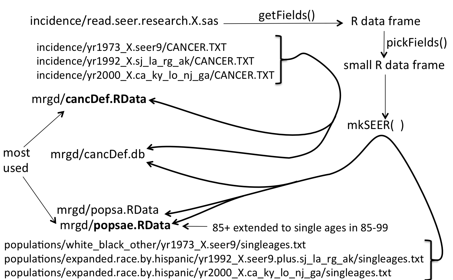
SEER data field positions and names change over the years and the original purpose of
SEERaBomb was to buffer/protect R scripts from such changes. A second purpose was to speed up SEER data computations by
reducing the data [via pickFields()] to only fields of interest. SEERaBomb now has an additional purpose:
estimating relative risks of SEER second cancers after diagnoses of first cancers, using all three SEER databases.
Note: SEER no longer includes radiation therapy data by default. Users must thus obtain custom SEER treatment data
https://seer.cancer.gov/data/treatment.html.
Details
| Package: | SEERaBomb |
| Type: | Package |
| Depends: | dplyr, ggplot2, rgl, demography |
| Suggests: | bbmle |
| License: | GPL-2 |
| LazyData: | yes |
| URL: | http://epbi-radivot.cwru.edu/SEERaBomb/SEERaBomb.html |
Author(s)
Tom Radivoyevitch (radivot@ccf.org)
References
Surveillance, Epidemiology, and End Results (SEER) Program (www.seer.cancer.gov) Research Data (1973-2015), National Cancer Institute, DCCPS, Surveillance Research Program, Surveillance Systems Branch, released April 2018, based on the November 2017 submission.
See Also
getFields,pickFields,mkSEER,mkSEERold,mkAbomb
Chromosome translocation versus age data
Description
This is chromosome translocation versus age data that is pooled across gender and race.
Usage
data(Sigurdson)Format
A data frame named Sigurdson with the following columns.
ageAge of donor of lymphocytes.
tlcnTotal number of chromosomal translocations per 100 cell equivalents.
Details
The data were obtained using FISH, see reference below. This dataset is loaded automatically with
library(SEERaBomb). As such, the function data() is not needed.
References
Sigurdson et al. Mutation Research 652 (2008) 112-121
Examples
library(SEERaBomb)
with(Sigurdson,plot(age,tlcn,cex=2,cex.axis=2,cex.lab=2,las=1,cex.main=2,
               ylab="",main="Translocations per 100 cells"))
Converts canc made by mkSEER into a data.frame with py at risk after firsts
Description
Makes a data frame in the exernal second cancer data format expected by esd.
Usage
canc2py(canc,firstS,secondS) Arguments
canc |
output of mkSEER |
firstS |
Charcter vector of first cancers of interest. |
secondS |
Charcter vector of second cancers of interest. |
Details
Use is currently limited to 2nd cancers in SEER since 1973, e.g. AML, since esd assumes its py column is in synch with times since diagnosis. This is not the case when e.g. MDS or CMML are in secondS.
Value
data.frame with columns: yrdx, agedx, sex, py at risk (in years), cancer1, and cancer2. Cases not ending in a second cancer have cancer2 set to "none".
Note
This function was developed with support from the Cleveland Clinic Foundation.
Author(s)
Tom Radivoyevitch (radivot@ccf.org)
See Also
Examples
## Not run:
rm(list=ls())
library(SEERaBomb)
load("~/data/SEER/mrgd/cancDef.RData")
secS=c("AML","MDS")
frstS=c("HL")
canc=canc%>%filter(cancer%in%union(frstS,secS))
load("~/data/SEER/mrgd/popsae.RData")
popsa=popsae%>%group_by(db,race,sex,age,year)%>%summarize(py=sum(py)) # sum on regs
pm=seerSet(canc,popsa,Sex="male",ageStart=0,ageEnd=100)
pf=seerSet(canc,popsa,Sex="female",ageStart=0,ageEnd=100)
pm=mk2D(pm,secondS=secS)
pf=mk2D(pf,secondS=secS)
brks=c(0,1,5,10)
pm=csd(pm,brkst=brks,firstS=frstS)
pf=csd(pf,brkst=brks,firstS=frstS)
S=rbind(pf$DF,pm$DF)%>%select(int,t,cancer1,cancer2,O,E) #merge sexes
S=S%>%group_by(int,cancer1,cancer2)%>%summarize(O=sum(O),E=sum(E),t=mean(t))
S=S%>%mutate(RR=O/E,rrL=qchisq(.025,2*O)/(2*E),rrU=qchisq(.975,2*O+2)/(2*E))
S$data="SEER"

ds=canc2py(canc,frstS,secS)
S2=esd(ds,pf$D,pm$D,brks)
S2=S2%>%group_by(int,cancer1,cancer2)%>%summarize(O=sum(O),E=sum(E),t=mean(t))
S2=S2%>%mutate(RR=O/E,rrL=qchisq(.025,2*O)/(2*E),rrU=qchisq(.975,2*O+2)/(2*E))
S2$data="SEER2"
d=rbind(S,S2)
d%>%filter(cancer1=="HL",cancer2=="AML")%>%arrange(int)
d%>%filter(cancer1=="HL",cancer2=="MDS")%>%arrange(int) #low because MDS not observable before 2001
yrcut=2001  # try to fix it like this
ds=ds%>%filter(yeaR+py>yrcut)
I=ds$yeaR<yrcut
ds$py[I]=(ds$py-(yrcut-ds$yeaR))[I]
S2=esd(ds,pf$D,pm$D,brks)
S2=S2%>%group_by(int,cancer1,cancer2)%>%summarize(O=sum(O),E=sum(E),t=mean(t))
S2=S2%>%mutate(RR=O/E,rrL=qchisq(.025,2*O)/(2*E),rrU=qchisq(.975,2*O+2)/(2*E))
S2$data="SEER2"
d=rbind(S,S2)
d%>%filter(cancer1=="HL",cancer2=="MDS")%>%arrange(int)
#the problem is that esd assumes that py is synched with tsx. csd handles the delays correctly.
d%>%filter(cancer1=="HL",cancer2=="MDS")%>%group_by(data)%>%summarize(o=sum(O)) #cases were shifted

## End(Not run)
Cancer risk vs years Since Diagnosis of other cancer
Description
Computes relative risks (RR) of 2nd cancers over specified intervals of times since diagnoses of a 1st cancer. 2D spline fits are used to produce expected cases E controlling for background risk dedepence on age and calendar year. RR is then O/E where O is the number of observed cases.
Usage
csd(seerSet,brkst=c(0),brksy=c(1975),brksa=c(0),trts=NULL,
                    PYLong=FALSE,firstS="all",exclUnkSurv=FALSE)
Arguments
seerSet |
A seerSet object produced by mk2D(). |
brkst |
Vector of breaks in years used to form Time intervals/bins since diagnosis. An upper limit of 100, well beyond 40 years of SEER follow up currently available, is assumed/added to brkst internally, and should thus not be in brkst. |
brksy |
Vector of breaks used to form groups of calendar Year at 1st cancer diagnosis intervals/bins. An upper limit of yearEnd (last year in SEER; a seerSet field) is assumed/added to brksy internally. |
brksa |
Vector of breaks used to form groups of Age at 1st cancer diagnosis intervals/bins. An upper limit of 126 is assumed. |
trts |
Character vector of treatments of interest. Default of NULL => all levels in seerSet's canc$trt. |
PYLong |
Set true if in addition to O and E for each tsd interval you also want PY strips for each individual; having these big dataframes slows saving seerSets, so only fetch if needed. |
firstS |
Character vector of first cancers of interest. Default of "all" sets it to the vector of all cancers in the seerSet field cancerS, which is created when the object is first created by seerSet(). |
exclUnkSurv |
Set true if you wish to exclude all cases with unknown survival times as a marker of bad data. |
Value
The input with an L component added to it or extended it if it already existed. Each component of L is a nested list of lists that can yield second cancer relative risks as a function of time since 1st cancer diagnosis. The most recent component of L is also provided as a data.frame seerSet$DF produced internally using getDF.
Note
This function was developed with support from the Cleveland Clinic Foundation.
Author(s)
Tom Radivoyevitch (radivot@ccf.org)
See Also
SEERaBomb-package, mk2D,seerSet
Examples
## Not run:
library(SEERaBomb)
pm=simSeerSet()
pm=mk2D(pm)
pm$canc
pm=csd(pm,brkst=c(0,5),brksy=c(1975,2000),brksa=c(0,50),trts=c("noRad","rad"))
pm
library(ggplot2)
theme_set(theme_gray(base_size = 16))
theme_update(legend.position = "top")
g=qplot(x=t,y=RR,data=subset(pm$DF,cancer1=="A"&cancer2=="B"),col=trt,geom=c("line","point"),
        xlab="Years Since First Cancer Diagnosis",ylab="Relative Risk")
g=g+facet_grid(yearG~ageG,scales="free")+geom_abline(intercept=1, slope=0)
g+geom_errorbar(aes(ymin=rrL,ymax=rrU,width=.15))

## End(Not run)
Event vs years Since Diagnosis
Description
Computes relative risks (RR) of second cancers over specified years-since-diagnosis intervals. SEER incidence rates are used to compute background/expected numbers of cases E, sex, age, and calendar year specifically. RR = O/E where O and E are the numbers of observed and expected cases.
Usage
esd(d,srfF,srfM,brkst=c(0,2,5),brksy=NULL) Arguments
d |
Input data.frame with columns: yrdx, agedx, sex, py at risk (in years), cancer1, and cancer2. Cancer1 and cancer2 should use standard SEERaBomb cancer names, see mapCancs. Cases not ending in a second cancer should have cancer2 set to "none". |
srfF |
Female incidence surface. Output D of mk2D for females, for cancers in cancer2 |
srfM |
Male incidence surface. Output D of mk2D for males, for cancers in cancer2 |
brkst |
Vector of breaks in years used to form times since diagnosis intervals/bins. |
brksy |
Vector of breaks of calendar years to show trends. Leave NULL for all in one. |
Value
data.frame with observed and expected cases, RR, and RR CI for each time since diagnosis interval.
Note
This function was developed with support from the Cleveland Clinic Foundation.
Author(s)
Tom Radivoyevitch (radivot@ccf.org)
See Also
Fills age-year person year (PY) matrix
Description
This internal function converts a matrix with lots of individual PY contributions and starting ages and years as rows, into a population-level PY histrogram matrix of (1-year age)x(1-year year) resolution bins. The output matrix is more square-like (currently at 40 calendar years by 126 age years) than the tall dataframe-like input matrix.
Usage
fillPYM(PYin,PYM)
Arguments
PYin |
Tall input matrix where rows hold individual PY at risk, year and starting (left) ages ageL. |
PYM |
Output PY matrix with age and calendar year rows and columns at single year resolution. |
Value
The second argument becomes the output. This matrix should be filled with zeros in R before calling this function. After the call, it will be filled; this function uses pointers in Rcpp C++ code.
Author(s)
Tom Radivoyevitch (radivot@ccf.org)
Examples
  yrs=1975:1990
  ages=0.5:70.5
  PYM=matrix(0,ncol=length(yrs),nrow=length(ages))
  colnames(PYM)=yrs
  rownames(PYM)=ages
(PYin=structure(c(3.5, 11.25,5.2, 51.5, 58.5,0.75, 1976, 1977,1980),.Dim = c(3L,3L),
                  .Dimnames=list(c("1","2","3"),c("py", "ageL", "year"))))
fillPYM(PYin, PYM)
Gets the lower and upper limit and index of a tsd bin
Description
Extract time since diagnosis (tsd) interval information in strings produced by cut.
Usage
getBinInfo(binLab, binS)Arguments
binLab |
The label of the specific bin of interest. |
binS |
The character vector of bin labels in which binLab exists. |
Value
A numeric vector containting the lower limit (LL), upper limit (UL), and position (index) in the parent vector binS.
Author(s)
Tom Radivoyevitch (radivot@ccf.org)
See Also
Examples
library(SEERaBomb)
brks=c(0,0.25,1,3,5)
(binS=levels(cut(brks+0.1,breaks=c(brks,100)))) #make a vector of intervals
getBinInfo(binS[4],binS) # test getBinInfo
Converts a seerSet$L series to a data.frame
Description
Creates a data.frame of observed and expected cases for each first and second cancer and treatment. csd() calls this internally for the most recent time series, so it may not need to be called directly.
Usage
getDF(seerSet,srs=NULL)Arguments
seerSet |
seerSet object produced by csd(). |
srs |
Series. The time series of interest. NULL (default) implies the currently active series, which is the most recent. A number i implies the ith series. A string identifies the series by name (numeric vectors will be coerced to such a string via paste0("b",paste(brks,collapse="_")) where brks = vector of time breakpoints. |
Value
A data.frame in long format that can be used by ggplot.
Note
I envision getting away from saving multiseries seerSet objects and instead just saving several DF outputs of getDF. Besides smaller objects, a reason for this is that two L objects out of csd can now be confounded if they have the same time since diagnosis series but a different series for age and/or year of diagnosis.
Author(s)
Tom Radivoyevitch (radivot@ccf.org)
See Also
Examples
## Not run:
library(SEERaBomb)
load("~/data/SEER/mrgd/cancDef.RData") #load in canc
load("~/data/SEER/mrgd/popsae.RData") # load in popsae
canc=canc%>%select(-reg,-recno,-agerec,-numprims,-COD,
          -age19,-age86,-radiatn,-ICD9,-db,-histo3)
popsa=popsae%>%group_by(db,race,sex,age,year)%>%summarize(py=sum(py)) # sum on regs
pm=seerSet(canc,popsa,Sex="male",ageStart=0,ageEnd=100) #pooled (races) male seerSet
pm=mk2D(pm,secondS=c("AML","MDS"))
firstS=c("NHL","MM")
pm=csd(pm,brkst=c(0,1,5),trts=c("rad","noRad"),firstS=firstS)
pm$DF
getDF(pm)

## End(Not run)
Get expected numbers of cases
Description
Converts list of matrices produced by post1PYO into a matrix that corresponds to the matrix of observed cases produced by post1PYO.
Usage
getE(LPYM,D,ageStart,ageEnd,yearEnd,firstS,secondS)Arguments
LPYM |
List of first cancer PY matrices produced by post1PYO. |
D |
D component of seerSet list produced by mk2D. |
ageStart |
ageStart component of seerSet. |
ageEnd |
ageEnd component of seerSet. |
yearEnd |
The most recent year in the SEER datasets. |
firstS |
Character vector of first cancers of interest; added to seerSet by tsd. |
secondS |
Character vector of second cancers of interest; added to seerSet by mk2D. |
Value
A matrix of expected cases with first cancers labeling the rows and second cancers labeling the columns.
Author(s)
Tom Radivoyevitch (radivot@ccf.org)
See Also
Examples
## Not run:
library(SEERaBomb)
pm=simSeerSet()
pm=mk2D(pm,secondS="B")
L=post1PYO(pm$canc,brks=c(0,2,5),binIndx=1,Trt="rad",yearEnd=2012 )
names(L)
names(pm)
with(pm,getE(L$LPYM,D,ageStart,ageEnd,yearEnd,cancerS,secondS))

## End(Not run)
Get fields from SEER SAS file
Description
Converts the SAS file in the SEER ‘incidence’ directory into a data frame in R.
Usage
getFields(seerHome="~/data/SEER")Arguments
seerHome |
The directory that contains the SEER ‘population’ and ‘incidence’ directories. |
Details
SEER provides a SAS file for reading SEER ASCII data files into SAS. This file is parsed by getFields() to generate a data frame in R that contains all of the SEER fields. This data frame describes these fields in terms of their names (short and long forms), their starting points, and their widths.
Value
A data frame with one row for each field and columns that contain corresponding starting positions, widths, sas names, short names, and expansions thereof.
Author(s)
Tom Radivoyevitch (radivot@ccf.org)
See Also
SEERaBomb-package, mkSEER, pickFields
Examples
## Not run:
library(SEERaBomb)
(df=getFields())
head(df,20)

## End(Not run)
Get tsd interval PY
Description
Gets person year (PY) contributions to a particular time since diagnosis (tsd) interval from survival times.
Usage
getPY(surv, bin, binS, brks)Arguments
surv |
The total survival time of the patient. |
bin |
The label of the specific bin of interest. |
binS |
The character vector of bin labels in which binLab exists. |
brks |
The numeric vector of break points used by cut to create binS. |
Value
A vector as long as the survival vector input of PY at risk in a particular interval.
Author(s)
Tom Radivoyevitch (radivot@ccf.org)
See Also
Examples
library(SEERaBomb)
brks=c(0,0.25,1,3,6)
(binS=levels(cut(brks+0.1,breaks=c(brks,100)))) #make a vector of intervals
survTimes=c(8,16,1.5,3.7)
getPY(survTimes,binS[1],binS,brks)# all contribute 0.25 to first interval
getPY(survTimes,binS[4],binS,brks)# 3rd and 4th survivals contribute 0 and 0.7 to (3,6]
getPY(survTimes,binS[5],binS,brks)# 1st and 2nd survival contribute 2 and 10 years to (6,100]
Computes A-bomb incidences
Description
Creates A-bomb survivor incidence rates and confidence intervals.
Usage
incidAbomb(d)Arguments
d |
Tibble, typically grouped, with DG column ending 1st block and py starting the last. |
Details
The columns DG and py must exist in d, in that order.
Person-year weighted means will be formed of any columns between them.
Its OK if none exist. Sums are formed on py and anything to their right. It is assumed
that cancer types begin after py, with at most upy and/or subjects intervening them.
Value
A tibble data frame, summarized by groups, with cancers after py in a new cancers column, and new columns O (observed cases), incid and incid 95% CI limits LL and UL.
Author(s)
Tom Radivoyevitch (radivot@ccf.org)
See Also
Computes SEER incidences
Description
Creates SEER incidence rates and confidence intervals.
Usage
incidSEER(canc,popsae,cancers)Arguments
canc |
data frame of cancer cases |
popsae |
data frame of person years at risk |
cancers |
character vector of cancer types |
Details
This left joins popsae and cancers in canc.
Value
A data frame with observed cases (O), incid, and incid 95% CI limits LL and UL.
Author(s)
Tom Radivoyevitch (radivot@ccf.org)
See Also
Map CODs to strings
Description
Maps integer cause of death (COD) codes in COD of a SEER cancer data frame to a factor CODS with recognizable levels. This is a bit slow, so it is called within mkSEER.
Usage
mapCODs(D)Arguments
D |
A data frame that includes COD as a column. |
Value
The input data frame with an additional CODS column added on.
Note
Typing mapCODs dumps the function definition and thus the mapping used.
Author(s)
Tom Radivoyevitch (radivot@ccf.org)
See Also
Examples
library(SEERaBomb)
mapCODs # shows default definitions
Map ICD9 and ICD-O3 codes to cancers
Description
Adds a factor cancer with easily recognizable levels to a SEER cancer data.frame.
Usage
mapCancs(D)Arguments
D |
A data frame that includes ICD9 and histo3 as columns. |
Value
The input data frame with an additional cancer column added on.
Note
This is used by mkSEER() when it generates R binaries of the SEER data. Otherwise it provides current cancer definitions (seen by looking at the function definition).
Author(s)
Tom Radivoyevitch (radivot@ccf.org)
See Also
Examples
library(SEERaBomb)
mapCancs # shows default definitions
Map registry codes to acronyms
Description
Maps codes for SEER registries to 2-letter acronyms and corresponding descriptions.
Usage
mapRegs(code=NA)Arguments
code |
Full SEER codes as found in SEER Cancer files. Add 1500 to popuation file codes get such cancer file codes. If this argument is missing (the default) a full dataframe of symbols and descriptions is returned. |
Value
A dataframe of SEER registry symbols and descriptions with rownames such as "1501" for sf (san francisco) and "1520" for dM (detroit Michigan), or just the symbol if the rowname is given. Note that city characters are in lower case and state characters are in upper case.
Note
This function is used by mkSEER when it generates merged R binaries. It is exposed to provide quick access to registry acronym definitions.
Author(s)
Tom Radivoyevitch (radivot@ccf.org)
See Also
Examples
library(SEERaBomb)
mapRegs(1501)
mapRegs()
Map treatment codes to factor
Description
Uses SEER codes in the SEER field radiatn to add a factor named trt with levels "noRad","rad", and "unk" to a cancer data frame.
Usage
mapTrts(D)Arguments
D |
A SEER cancer data frame that includes the field radiatn as a column. |
Value
The input data frame with an additional trt column added to its end.
Note
This function is used by mkSEER when it generates merged R binaries. It is exposed to state the default definition of trt and, by way of example, to show how to override it.
Author(s)
Tom Radivoyevitch (radivot@ccf.org)
See Also
Examples
library(SEERaBomb)
mapTrts # exposes default definition of trt
Make 2D-spline fits of incidences
Description
Produces two dimensional (2D) spline fits of cancer incidence versus age and calendar year, with interactions. In conjunction with person years (PY) at risk, this is used in csd() to produce expected numbers of cases under a null hypothesis that prior cancers do not impact subsequent cancer risks.
Usage
mk2D(seerSet, knots=5, write=FALSE, outDir="~/Results",txt=NULL,secondS=NULL)Arguments
seerSet |
Object of class seerSet, i.e. output list of seerSet(). |
knots |
Base number of knots; overrides are in place for some cancers. |
write |
TRUE = write 2D fits to files. The fits can be >300 MB and take >60 seconds to write, so leave FALSE unless you need it. |
outDir |
Folder that will hold the output files. |
txt |
Additional text to distinguish files with different cancer lists. This may be useful during spline fit development. |
secondS |
Charcter vector of second cancers of interest (note: I often capitalize the final S of vectors of Strings). |
Value
The input seerSet with an additional data frame D added to this list. D holds background/expected incidences over a 1-year resolution age-year grid.
Author(s)
Tom Radivoyevitch (radivot@ccf.org)
See Also
SEERaBomb-package, plot2D, seerSet
Examples
## Not run:
library(SEERaBomb)
(pm=simSeerSet())
(pm=mk2D(pm))
names(pm)
head(pm$D)
tail(pm$D)

## End(Not run)
Make Abomb Binaries
Description
Converts Abomb files ‘lsshempy.csv’ and ‘lssinc07.csv’
into tibbles heme and solid in the file ‘abomb.RData’.
Usage
mkAbomb(AbombHome="~/data/abomb")Arguments
AbombHome |
Directory with Abomb files. Should be writable by user. |
Details
The files ‘lsshempy.csv’ and ‘lssinc07.csv’ can be found under The incidence of leukemia, lymphoma and multiple myeloma among atomic bomb survivors: 1950-2001 and Life Span Study Cancer Incidence Data, 1958-1998 of the Radiation Effects Research Foundation (RERF) website http://www.rerf.or.jp/.
Value
None. This function is called for its side-effect of producing ‘abomb.RData’.
Author(s)
Tom Radivoyevitch (radivot@ccf.org)
See Also
Examples
## Not run:
library(SEERaBomb)
mkAbomb()
load("~/data/abomb/abomb.RData")
View(heme)

## End(Not run)
Converts seerSet$L series to a data.frame
Description
Creates a data.frame of observed and expected cases for each first and second cancer and treatment. Use of this function is deprecated. Use getDF() instead, if needed: csd now calls getDF internally for the most recent time series, so even it may not need to be called directly.
Usage
mkDF(seerSet,srs)Arguments
seerSet |
seerSet object produced by tsd(). |
srs |
Series. The time series of interest. NULL (default) implies the currently active series, which is the most recent. A number i implies the ith series. A string identifies the series by name (numeric vectors will be coerced to such a string via paste0("b",paste(brks,collapse="_")) where brks = vector of time breakpoints. |
Value
A data.frame in long format that can be used by ggplot.
Author(s)
Tom Radivoyevitch (radivot@ccf.org)
See Also
Examples
## Not run:
library(SEERaBomb)
load("~/data/SEER/mrgd/cancDef.RData") #load in canc
load("~/data/SEER/mrgd/popsae.RData") # load in popsae
canc=canc%>%select(-reg,-recno,-agerec,-numprims,-COD,
          -age19,-age86,-radiatn,-ICD9,-db,-histo3)
popsa=popsae%>%group_by(db,race,sex,age,year)%>%summarize(py=sum(py)) # sum on regs
pm=seerSet(canc,popsa,Sex="male",ageStart=0,ageEnd=100) #pooled (races) male seerSet
pm=mk2D(pm,secondS=c("AML","MDS"))
brks=c(0,1,5)
firstS=c("NHL","MM")
pm=tsd(pm,brks=brks,trts=c("rad","noRad"),firstS=firstS)
mkDF(pm)

## End(Not run)
Make Demographics Tables
Description
Provides, in an Excel file, quartiles of age at diagnoses in one sheet and median overall survival times on a second. Many tables are placed in each sheet. One Excel file is produced per cancer type.
Usage
mkDemographics(canc,outDir="~/Results/SEERaBomb")Arguments
canc |
A dataframe that includes cancer, age at diagnosis (agedx), age (grouped agedx), race, sex, year (grouped), COD, surv, and trt. |
outDir |
Folder of the Excel file(s) that will be generated. |
Value
Returned invisibly is a list of data frames corresponding to tables of the Excel file(s).
Author(s)
Tom Radivoyevitch (radivot@ccf.org)
See Also
Examples
## Not run:
library(SEERaBomb)
rm(list=ls())
load("~/data/SEER/mrgd/cancDef.RData")
canc$year=cut(canc$yrdx,c(1973,2003,2009,2015),include.lowest = T,dig.lab=4)
canc$age=cut(canc$agedx,c(0,40,50,60,70,80,90,126),include.lowest = T)
canc=canc%>%filter(surv<9999)
canc=canc%>%select(-age86,-radiatn,-chemo,-db,-casenum,-modx,-seqnum,-yrbrth,-ICD9,-reg,-histo3)
canc=canc%>%filter(cancer%in%c("AML","MDS","MPN"))
head(canc,3)
mkDemographics(canc)

## End(Not run)
Make RR Excel file from csd output
Description
Provides relative risks (RR) organized by 1st and 2nd cancers, times since 1st cancer diagnoses, and 1st cancer treatment. RR = O/E where O = observed cases and E = cases expected under a null hypothesis that prior cancers do not impact subsequent risks. If flip = FALSE (default), sheets = 1st cancers and rows = 2nd cancers, else sheets = 2nd cancers and rows = 1st cancers; columns are always intervals of years since diagnosis, in 1st cancer treatment blocks. RR CI and observed numbers are included in each data cell.
Usage
mkExcelCsd(seerSet,tsdn,biny="[1975,2017)",bina="(0,126]",
                        outDir="~/Results",outName=NULL,flip=FALSE)
Arguments
seerSet |
A seerSet list after it has been processed by csd(). |
tsdn |
Name of set of times since diagnosis. This is based on the brkst argument to csd(). If length >1 a brkst vector is assumed and coerced/collapsed to a tsdn string. |
biny |
Year at DX interval. |
bina |
Age at DX interval. |
outDir |
Folder of the Excel file that will be generated. |
outName |
if null (default), Excel file name = seerSet base file name (bfn) + tsdn, else it is outName. Eitherway, "Flipped" is appended to the name if flip is TRUE. |
flip |
If FALSE, sheets are first cancers, rows seconds. If TRUE, sheets are second cancers, rows firsts. |
Value
Returned invisibly, a list of data frames corresponding to sheets of the Excel file.
Note
Outputs are for a given sex. Races are typically pooled.
Author(s)
Tom Radivoyevitch (radivot@ccf.org)
See Also
SEERaBomb-package, mk2D,seerSet
Examples
## Not run:
library(SEERaBomb)
pm=simSeerSet()
pm=mk2D(pm)
mybrks=c(0,1,5,10)
pm=csd(pm,brkst=mybrks,trts=c("noRad","rad"))
(lab=paste0("b",paste(mybrks,collapse="_")))
(L=mkExcelCsd(pm,lab))
(L=mkExcelCsd(pm,lab,flip=TRUE))

## End(Not run)
Make RR Excel file from tsd function output
Description
Provides relative risks (RR) organized by 1st and 2nd cancers, times since 1st cancer diagnoses, and 1st cancer treatment. RR = O/E where O = observed cases and E = cases expected under a null hypothesis that prior cancers do not impact subsequent risks. If flip = FALSE (default), sheets = 1st cancers and rows = 2nd cancers, else sheets = 2nd cancers and rows = 1st cancers; columns are always intervals of years since diagnosis, in 1st cancer treatment blocks. RR CI and observed numbers are included in each data cell.
Usage
mkExcelTsd(seerSet,tsdn,outDir="~/Results",outName=NULL,flip=FALSE)Arguments
seerSet |
A seerSet list after it has been processed by tsd(). |
tsdn |
Name of set of times since diagnosis. This is based on the brks argument to tsd(). If length >1 a brkst vector is assumed and coerced/collapsed to a tsdn string. |
outDir |
Folder of the Excel file that will be generated. |
outName |
if null (default), Excel file name = seerSet base file name (bfn) + tsdn, else it is outName. Eitherway, "Flipped" is appended to the name if flip is TRUE. |
flip |
If FALSE, sheets are first cancers, rows seconds. If TRUE, sheets are second cancers, rows firsts. |
Value
Returned invisibly, a list of data frames corresponding to sheets of the Excel file.
Note
Outputs are for a given sex. Races are typically pooled.
Author(s)
Tom Radivoyevitch (radivot@ccf.org)
See Also
SEERaBomb-package, mk2D,seerSet
Examples
## Not run:
library(SEERaBomb)
pm=simSeerSet()
pm=mk2D(pm)
mybrks=c(0,1,5,10)
pm=tsd(pm,brkst=mybrks,trts=c("noRad","rad"))
(lab=paste0("b",paste(mybrks,collapse="_")))
(L=mkExcelTsd(pm,lab))
(L=mkExcelTsd(pm,lab,flip=TRUE))

## End(Not run)
Make Life Tables
Description
Makes life tables from mortality data binaries produced by mkMrt() and places the files in the same folder.
Usage
mkLT(mrtHome="~/data/usMort",input="mrt.RData",output="ltb.RData")Arguments
mrtHome |
Directory that contains the mortality data binary. |
input |
File that contains the mortality data binary. |
output |
File that will contain the life tables. |
Value
None. This function is called for its side-effect of producing male and female life tables in files.
Author(s)
Tom Radivoyevitch (radivot@ccf.org)
See Also
Examples
## Not run:
library(SEERaBomb)
mkLT()
load("~/data/usMort/ltb.RData")
tail(ltb$Female)

## End(Not run)
Make mortality binaries
Description
Gets mortality data from the Human Mortality Database http://www.mortality.org/ and puts it in the file ‘mrt.RData’.
Usage
mkMrt(username,passwd,country="USA",mrtHome="~/data/usMort")Arguments
username |
Username of Human Mortality Database account. |
passwd |
Password of Human Mortality Database account. |
country |
This should probably stay at its default of USA. |
mrtHome |
Directory that will contain the mortality data binary. Should be writable by user. |
Value
None. This function is called for its side-effect of producing ‘mrt.RData’.
Author(s)
Tom Radivoyevitch (radivot@ccf.org)
References
Barbieri M, Wilmoth JR, Shkolnikov VM, et al. Data Resource Profile: The Human Mortality Database (HMD). Int J Epidemiol. 2015;44: 1549-1556.
See Also
Examples
## Not run:
library(SEERaBomb)
mkMrt("username", "password")# sub in your personal account info
load("~/data/usMort/mrt.RData")
head(mrt$Female)

## End(Not run)
Make mortality binaries from local HMD data files
Description
Converts locally installed Human Mortality Data http://www.mortality.org/ into an R binary file ‘mrtCOUNTRY.RData’.
Usage
mkMrtLocal(country="USA",mrtHome="~/data/mrt",
                    mrtSrc1="~/data/hmd_countries",
                    mrtSrc2="~/data/hmd_statistics/death_rates/Mx_1x1"
                    )
Arguments
country |
Default is USA. See names of subfolders of ‘hmd_countries’ for other options. |
mrtHome |
Directory that will contain the mortality data binary. Should be writable by user. |
mrtSrc1 |
Directory with hmd_countries data (first choice of files = "all HMD countries"). |
mrtSrc2 |
Directory with hmd_statistics data (second choice of files = "all HMD statistics"). |
Value
None. This function is called for its side-effect of producing ‘mrt.RData’ from HMD files organized as all HMD countries or all HMD statistics on the HMD download page (you need at least one of these).
Author(s)
Tom Radivoyevitch (radivot@ccf.org)
References
Barbieri M, Wilmoth JR, Shkolnikov VM, et al. Data Resource Profile: The Human Mortality Database (HMD). Int J Epidemiol. 2015;44: 1549-1556.
See Also
Examples
## Not run:
library(SEERaBomb)
mkMrtLocal()
load("~/data/mrt/mrtUSA.RData")
head(mrt$Female)

## End(Not run)
Make R binaries of SEER data.
Description
Converts SEER ASCII text files into large R binaries that include all cancer types and registries combined.
Usage
mkSEER(df,seerHome="~/data/SEER",outDir="mrgd",outFile="cancDef",
                  indices = list(c("sex","race"), c("histo3","seqnum"),  "ICD9"),
                  writePops=TRUE,writeRData=TRUE,writeDB=FALSE)
Arguments
df |
A data frame that was the output of |
seerHome |
The directory that contains the SEER ‘population’ and ‘incidence’ directories. This should be writable by the user. |
outDir |
seerHome subdirectory to write to. Default is ‘mrgd’ for all registries merged together. |
outFile |
Base name of the SQLite database and cancer binary. Default = cancDef (Cancer Default). |
indices |
Passed to |
writePops |
TRUE if you wish to write out the population data frame binaries. Doing so takes ~10 seconds, so savings of FALSE are small. |
writeRData |
TRUE if you wish to write out the cancer data frame binary. Writing files takes most of the time. |
writeDB |
TRUE if you wish to write cancer, popga, popsa, and popsae data frames to SQLite database tables. |
Details
This function uses the R package LaF to access the fixed-width format data files
of SEER. LaF is fast, but it requires knowledge of all the widths of columns wanted, as well as the the widths of unwanted stretches in between. This knowledge is produced by getFields() and pickFields() combined. It is passed to mkSEER() via the argument df.
Value
None, it produces R binary files of the SEER data.
Note
This takes a substantial amount of RAM (it works on a Mac with 16 GB of RAM) and time (~3 minutes using default fields).
Author(s)
Tom Radivoyevitch (radivot@ccf.org)
See Also
SEERaBomb-package,getFields,pickFields
Examples
## Not run:
library(SEERaBomb)
(df=getFields())
(df=pickFields(df))
# the following will take a several minutes, but may only need
# to be done roughly once per year, with each release.
mkSEER(df)

## End(Not run)
Make SEER binaries as before
Description
Converts SEER ASCII text files into smaller R binaries. This is being maintained to avoid fixing old scripts. Please use mkSEER for new scripts.
Usage
mkSEERold(df,seerHome="~/data/SEER",
            dataset=c("00","73","92"),SQL=TRUE, mkDFs=FALSE)
Arguments
df |
A data frame that was the output of |
seerHome |
The directory that contains the SEER ‘population’ and ‘incidence’ directories. This should be writable by the user. |
dataset |
The SEER database to use, specified as a string of the last two digits of the starting year, i.e. |
SQL |
TRUE if an SQLite database is to be created. The file ‘all.db’ produced in this case can be significantly larger than the sum of the ‘*.RData’ files also produced. |
mkDFs |
TRUE if you wish to make data frame binaries. |
Details
See mkSEER.
Value
None. This function produces R binary data files.
Author(s)
Tom Radivoyevitch (radivot@ccf.org)
See Also
SEERaBomb-package,mkSEER,getFields,pickFields
Examples
## Not run:
library(SEERaBomb)
(df=getFields())
(df=pickFields(df))
for (i in c("73","92","00")) mkSEERold(df,dataset=i)

## End(Not run)
Mortality vs years Since Diagnosis
Description
Computes relative risks (RR) of death over specified years-since-diagnosis intervals. US mortality rates obtained via the R package demography are used to compute background death dedepence on age and calendar year. RR is then O/E where O and E are the number of observed and expected cases.
Usage
msd(canc,mrt,brkst=c(0,2,5),brksy=NULL) Arguments
canc |
Input data.frame with columns: yrdx, agedx, sex, surv (in years), and status (1=dead). |
mrt |
List with male and female fields, each matrices with mortality rates vs year and age. |
brkst |
Vector of breaks in years used to form Times since diagnosis intervals/bins. |
brksy |
Vector of breaks of calendar Years to show mortality trends. Leave NULL for all in one. |
Value
data.frame with observed and expected cases, RR, and RR CI for each tsd interval.
Note
This function was developed with support from the Cleveland Clinic Foundation.
Author(s)
Tom Radivoyevitch (radivot@ccf.org)
See Also
SEERaBomb-package, mk2D,seerSet
Examples
## Not run:
library(SEERaBomb)
load("~/data/SEER/mrgd/cancDef.RData") #loads in canc
lu=canc%>%filter(cancer=="lung")
lu=lu%>%mutate(status=as.numeric(COD>0))%>%select(yrdx,agedx,sex,surv,status)
lu=lu%>%mutate(surv=round((surv+0.5)/12,3))#convert surv to years

# library(demography)
# d=hmd.mx("USA", "username", "password") #make an account and put your info in here
# mrt=d$rate
# save(mrt,file="~/data/usMort/mrt.RData")
load("~/data/usMort/mrt.RData"); object.size(mrt)# 250kb
brks=c(0,0.5,3,6,10,15,20,25)
(dlu=msd(lu,mrt,brkst=brks))

## End(Not run)
National Vital Statistic Report (nvsr) Data
Description
US mortality rates (probability of death that year) in 2010; report published Nov. 2014.
Usage
nvsr
Format
A data frame with the following columns.
ageSingle-year resolution ages up to 99.5.
pPooled sexes and races.
pmPooled races, males.
pfPooled races, females.
wWhites, sexes pooled.
bBlacks, sexes pooled.
oOthers, sexes pooled.
wmWhite males.
wfWhite females.
bmBlack males.
bfBlack females.
omOther males.
ofOther females.
References
National Vital Statistics Reports, Vol. 63, No. 7, November 6, 2014 http://www.cdc.gov/nchs/data/nvsr/nvsr63/nvsr63_07.pdf
Examples
library(SEERaBomb)
head(nvsr)
National Vital Statistic Report (nvsr01) Data
Description
US mortality rates (probability of death that year) in 2001 (Report 52_14).
Usage
nvsr01
Format
A data frame with the following columns.
ageSingle-year resolution ages up to 99.5.
pPooled sexes and races.
pmPooled races, males.
pfPooled races, females.
wmWhite males.
wfWhite females.
bmBlack males.
bfBlack females.
Details
This data is used to extrapolate PY at risk in SEER population files from 85+ to older ages.
References
ftp://ftp.cdc.gov/pub/Health_Statistics/NCHS/Publications/NVSR/52_14/
Examples
library(SEERaBomb)
head(nvsr01)
Primary to Secondary
Description
Using a SEER data frame, this function computes times between primary and secondary cancers. In the resulting data frame, surv and status can be analyzed at the individual level, e.g. using Cox regression.
Usage
p2s(canc,firstS,secondS,yrcut=2010) Arguments
canc |
Data frame produced by mkSEER(). |
firstS |
Vector of names (as Strings) of first cancers you wish to consider. |
secondS |
Vector of names of second cancers you wish to consider. |
yrcut |
Only cases diagnosed in yrcut or newer are analyzed. The default of 2010 is the year AML cases after MDS began to be entered into SEER as second cancers; before they were considered to be part of the first cancer. This function facilitates studies of the rate at which myeloid neoplasms such as MDS progress to AML. |
Value
Data frame with a row for each primary (first cancer) diagnosed on or after yrcut. The surv column holds the time in months to last follow up or death (status=0), or to the time of diagnosis of the second cancer (status=1).
Author(s)
Remco J. Molenaar (r.j.molenaar@amc.uva.nl )
See Also
SEERaBomb-package, mk2D,seerSet
Examples
## Not run:
#

## End(Not run)
Pick SEER fields of interest
Description
Reduces the full set of SEER data fields to a smaller set of interest. SEER fields
are rows of the input and output dataframes
of this function. The output dataframe differs from the input dataframe not only in there being fewer rows
but also in there being an additional column needed by mkSEER() downstream.
Usage
pickFields(sas,picks=c("casenum","reg","race","sex","agedx",
        "yrbrth","seqnum","modx","yrdx","histo3",
        "ICD9","COD","surv","radiatn","chemo"))
Arguments
sas |
A data frame created by |
picks |
Vector of names of variables of interest. This set should not be smaller than the default. |
Details
R binaries become too large if all of the fields are selected. SEERaBomb is faster than SEER*Stat
because it tailors/streamlines the database to your interests. The default picks are a reasonable place to start; if you
determine later that you need more fields, you can always rebuild the binaries. Grabbing all fields is
discouraged, but if you want this anyway, note that you still need pickFields() to create a data type column, i.e. you cannot bypass pickFields() by sending the output of getFields() straight to mkSEER().
Value
The SAS-based input data frame sas, shortened to just the rows of picks, and expanded to include
spacer rows of fields of no interest pooled into single strings: the width of such a spacer row is equal to
the distance in bytes between the fields of interest above and below it. This data frame is then
used by laf_open_fwf() of LaF in mkSEER() to read the SEER files. Proper use of this function, and of the SEER data in general,
requires an understanding of the contents of ‘seerdic.pdf’ in the ‘incidence’ directory of seerHome.
Author(s)
Tom Radivoyevitch (radivot@ccf.org)
See Also
SEERaBomb-package, getFields, pickFields, mkSEER
Examples
## Not run:
library(SEERaBomb)
(df=getFields())
(df=pickFields(df))


## End(Not run)
Plot 2D cancer incidence splines
Description
Plots splines of incidence versus age and calendar year produced by mk2D.
Usage
plot2D(seerSet, write=TRUE,outDir="~/Results/plots",col="red")Arguments
seerSet |
seerSet object after it is processed by mk2D. |
write |
TRUE if you want to write images to a seerSet subfolder. The name of this subfolder is the basefilename (bfn) of the seerSet. |
outDir |
Parent folder of seerSet subfolders. |
col |
Color of surface plot. |
Details
A plot will be produced for each cancer fitted by mk2D. For the first of these, RGL will open a new X11 window. Adjustments of size and angle of this first plot will hold for all subsequent plots. After each plot, the user hits any key to write the plot to a file and advance through the list of cancers.
Value
None, results go to the screen and to png files.
Author(s)
Tom Radivoyevitch (radivot@ccf.org)
See Also
SEERaBomb-package, mk2D,seerSet
Examples
## Not run:
library(SEERaBomb)
n=simSeerSet()
n=mk2D(n)
plot2D(n)

## End(Not run)
Get person-years at risk and observed cases after first cancers
Description
Converts a canc data.frame into a list of objects containing information regarding person years at risk for a second cancer after having a first cancer, and the number observed, in a defined time since exposure interval and after a defined first cancer therapy.
Usage
post1PYO(canc, brks=c(0,2,5),binIndx=1,Trt="rad",PYLong=FALSE,yearEnd,firstS,secondS)Arguments
canc |
Input canc data.frame that is already sex, and possibly race, specific, but not cancer specific, as treatment of any first cancer could potentially cause any second cancer. |
brks |
A vector of break points in years used to form time since diagnosis bins. |
binIndx |
The index of the interval for which py are to be computed by calling this function. |
Trt |
The treatment for the first cancers. Note that the second cancer treatment is irrelevant here, so the input canc must not be reduced to only certain treatment types. |
PYLong |
PYLong of tsd. |
yearEnd |
This is taken from the seerSet object. |
firstS |
Vector of first cancers of interest as strings. |
secondS |
Vector of second cancers of interest as strings. |
Value
A list where the first element is a list LPYM with as many PY matrices (PYM) as cancers in canc. The second element is a matrix of cases observed in this interval after this treatment, where row names are first cancers and column names are second cancers. The third element is a trivial scalar, the py-weighted midpoint of the time interval selected.
Note
After the SEER data is installed, see the script mkRRtsx.R in the examples folder.
Author(s)
Tom Radivoyevitch (radivot@ccf.org)
See Also
SEERaBomb-package, getE,seerSet
Get person-years at risk and observed cases after first cancers
Description
Converts a canc data.frame into a list of objects containing information regarding person years at risk for a second cancer after having a first cancer, and the number observed, in defined intervals of time since diagnosis, calendar year, and age at diagnosis.
Usage
post1PYOc(canc, brkst=c(0),binIndxt=1,brksy=c(1973),binIndxy=1,brksa=c(0),binIndxa=1,
             Trt="rad",PYLong=FALSE,yearEnd,firstS,secondS)
Arguments
canc |
Input canc data.frame that is already sex, and possibly race, specific, but not cancer specific, as treatment of any first cancer could potentially cause any second cancer. |
brkst |
Vector of breaks in years used to form tsd intervals/bins. An upper limit of 100, well beyond 40 years of SEER follow up currently available, is assumed/added to brkst internally, and should thus not be in brkst. |
binIndxt |
The index of the tsd interval for which py are to be computed by calling this function. |
brksy |
Vector of breaks used to form groups of calendar year at diagnosis intervals/bins. An upper limit of yearEnd (last year in SEER; a seerSet field) is assumed/added to brksy internally. |
binIndxy |
The index of the year interval for which py are to be computed by calling this function. |
brksa |
Vector of breaks used to form groups of age at diagnosis intervals/bins. An upper limit of 126 is assumed. |
binIndxa |
The index of the age at DX interval for which py are to be computed by calling this function. |
Trt |
The treatment for the first cancers. Note that the second cancer treatment is irrelevant here, so the input canc must not be reduced to only certain treatment types. |
PYLong |
PYLong of tsd. |
yearEnd |
This is taken from the seerSet object. |
firstS |
Vector of first cancers of interest as strings. |
secondS |
Vector of second cancers of interest as strings. |
Value
A list where the first element is a list LPYM with as many PY matrices (PYM) as cancers in canc. The second element is a matrix of cases observed in this interval after this treatment, where row names are first cancers and column names are second cancers. And after a few other slots, the last element is a trivial scalar, the py-weighted midpoint of the time interval selected.
Author(s)
Tom Radivoyevitch (radivot@ccf.org)
See Also
SEERaBomb-package, getE,seerSet
Get person-years at risk and observed deaths after cancer
Description
Converts data.frame D into a list of objects containing information regarding person years at risk of death after cancer and the number of deaths observed, in a defined time since exposure interval.
Usage
post1PYOm(D,brks=c(0,2,5),binIndx=1,yearEnd)Arguments
D |
Input data.frame with columns: yrdx, agedx, surv, and status (1=dead). |
brks |
A vector of break points in years used to form time since diagnosis bins. |
binIndx |
The index of the interval for which py are to be computed by calling this function. |
yearEnd |
The most recent year of available mortality data. |
Value
A list where the first element is a PY matrix (PYM), the second element is a vector of deaths observed in the intervals, and the third is a scalar, the py-weighted midpoint of the time intervals.
Author(s)
Tom Radivoyevitch (radivot@ccf.org)
See Also
SEERaBomb-package, getE,post1PYO
Prints seerSet.summary objects
Description
Renders data.frame of cases and median ages and survival times with a title above and notes below it. Also qplots PY versus years.
Usage
## S3 method for class 'seerSet.summary'
print(x, ...)
Arguments
x |
seerSet.summary object produced by summary.seerSet(). |
... |
Included to match arg list of generic print. |
Value
None.
Author(s)
Tom Radivoyevitch (radivot@ccf.org)
See Also
SEERaBomb-package, summary.seerSet, seerSet
Examples
## Not run:
library(SEERaBomb)
load("~/data/SEER/mrgd/cancDef.RData") #load in canc
load("~/data/SEER/mrgd/popsae.RData") # load in popsae
canc=canc%>%select(casenum,race:histo3,surv,cancer,trt,id)
popsa=popsae%>%group_by(db,race,sex,age,year)%>%summarize(py=sum(py)) # sum on regs
pm=seerSet(canc,popsa,Sex="male",ageStart=0,ageEnd=100) #pooled (races) male seerSet
pm # no print method for seerSet object, so we see the list
summary(pm) # print method for summary renders the summary and a plot of PY

## End(Not run)
Second cancer risk vs attained age after first cancer
Description
Computes absolute risk of 2nd cancers as a function of attained age after first cancer.
Usage
riskVsAge(canc,firstS=c("NHL","HL","MM"),
                secondS=c("AML","MDS"),brksa=c(0,30,50,60,70,80))
Arguments
canc |
canc made by mkSEER(). |
firstS |
Character vector of first cancers of interest. |
secondS |
Character vector of second cancers of interest. |
brksa |
Vector of breaks in years used to form attained age intervals. |
Value
data.frame with incidence vs age.
Note
This function was developed with support from the Cleveland Clinic Foundation.
Author(s)
Tom Radivoyevitch (radivot@ccf.org)
See Also
Join SEER cancers and PY
Description
Creates a sex-specific list of cancer and population person year (PY) data frames, possibly specific to a race and interval of ages at diagnosis.
Usage
seerSet(canc,popsa,Sex, Race="pooled",ageStart=15,ageEnd=85)Arguments
canc |
Data frame of cancers that includes agedx, sex, race, yrdx, modx, surv and cancer. |
popsa |
Data frame of population PY at 1-year age resolution. |
Sex |
"male" or "female". |
Race |
"white", "black", "other", or "pooled" (default). |
ageStart, ageEnd |
canc and popsa will be reduced to ages in ageEnd>age>=ageStart. |
Details
In the output: 1) 0.5 years is added to ages at diagnosis (agedx) to reverse SEER flooring to integers; 2) 0.5 months is added to survival months (again, to reverse flooring) before dividing by 12 to convert to years; 3) year of diagnosis integers are converted to reals by adding to them the month of diagnosis (modx) - 0.5 divided by 12 (note that a modx of 1 represents anytime in the month of January). If ageEnd>85, popsae (extended to ages up to 99) should be used as the input for popsa. If popsa is used, the age86 column of popsa will be replaced by an age column. The age86 and yrbrth columns of a canc are not used and will be removed if they happen to be present; users should manually remove any other columns not needed to minimize seerSet object sizes. Sex and race columns in inputs are removed from outputs as they are specified in other (scalar) seerSet elements. Also removed from canc are cancer factor levels not present for that sex.
Value
A list containing sex specific subsets of canc and popsa and information regarding how they were reduced.
Author(s)
Tom Radivoyevitch (radivot@ccf.org)
See Also
SEERaBomb-package, mk2D, plot2D
Examples
## Not run:
library(SEERaBomb)
simSeerSet() # without data, a simulated seerSet
#  else, with data ...
load("~/data/SEER/mrgd/cancDef.RData") #load in canc
load("~/data/SEER/mrgd/popsae.RData") # load in popsae
# trim columns
library(dplyr)
canc=canc%>%select(-reg,-recno,-agerec,-numprims,-COD,
          -age19,-age86,-radiatn,-ICD9,-db,-histo3)
popsae=popsae%>%select(-reg,-db)
seerSet(canc,popsae,Sex="male",ageStart=0,ageEnd=100)

## End(Not run)
Summarize SEER data.
Description
Shows numbers of cases per cancer in each SEER database and PY in each registry. Sexes are pooled.
Usage
seerStats(canc,popsa)Arguments
canc |
Data frame of cancers that includes agedx and cancer columns. |
popsa |
Data frame of population PY at 1-year age resolution. |
Value
A list of 2 data.frames with sexes pooled, one of cases with cancer types as rows and as columns, databases, totals, cases >=100 years old or not, and numbers of first-, second-, third- and higher cancers. The second data.frame holds population PY, and PY-weighted ages, per registry.
Author(s)
Tom Radivoyevitch (radivot@ccf.org)
See Also
SEERaBomb-package, mk2D, plot2D
Examples
## Not run:
library(SEERaBomb)
load("~/data/SEER/mrgd/cancDef.RData") #load in canc
load("~/data/SEER/mrgd/popsae.RData") # load in popsae
seerStats(canc,popsae)

## End(Not run)
Simulate SEER cancers and population person years
Description
Simulates data for two cancers, A and B.
Usage
simSeerSet(N=2e9,yearEnd=2016,ka=1e-5,kb=0.04,Ab=1e-5,
                 tauA=10,tauB=1,delay=1,period=4)
Arguments
N |
Number of person years to simulate. Default is roughly that of SEER. |
yearEnd |
Most recent SEER year to simulate. |
ka |
Rate at which cancer A incidence increases linearly with age. |
kb |
Exponential aging rate constant for cancer B incidence. |
Ab |
Exponential amplitude for cancer B incidence. |
tauA |
Survival mean in years for cancer A. |
tauB |
Survival mean in years for cancer B. |
delay |
Years until the beginning of the excess risk of B. |
period |
Duration in Years of the excess risk of B. |
Value
A simulated seerSet object with popsa filled using US 2000 Std population proportions and canc with
cancers A and B
where the incidence of A increases linearly with age and B increase exponentially in age.
Survival times are assumed to be exponentially distributed with means of tauA years for A and tauB years for B.
Radiation therapy of A is assumed to increase RR of B to 5 uniformly for period years after delay years.
Note
Supported by the Cleveland Clinic Foundation.
Author(s)
Tom Radivoyevitch (radivot@ccf.org)
See Also
SEERaBomb-package, seerSet,mk2D, plot2D
Examples
## Not run:
library(SEERaBomb)
n=simSeerSet()
n=mk2D(n,secondS="B")
mybrks=c(0,0.75,0.9,1.1,1.25,2,2.5,3,3.5,4,4.75,4.9,5.1,5.25,6)
n=tsd(n,brks=mybrks,trts=c("rad","noRad"))
D=mkDF(n)%>%filter(cancer1=="A")%>%select(t,RR,L=rrL,U=rrU,trt)
head(D,2)
library(ggplot2)
theme_update(legend.position = c(.8, .815),
             axis.text=element_text(size=rel(1.2)),
             axis.title=element_text(size=rel(1.3)),
             legend.title=element_text(size=rel(1.2)),
             legend.text=element_text(size=rel(1.2)))
g=qplot(x=t,y=RR,col=trt,data=D,geom=c("line","point"),
        xlab="Years Since First Cancer Diagnosis",ylab="Relative Risk")
g+geom_abline(intercept=1, slope=0)+geom_errorbar(aes(ymin=L,ymax=U,width=.05))

## End(Not run)
Simulate Survival Times
Description
Uses background mortality rates to simulate background survival time for matching sex, age and year.
Usage
simSurv(d,mrt,rep=1,ltb=NULL,unif=TRUE)Arguments
d |
Data frame containing sex, agedx, yrdx, surv, and status columns of observed data. |
mrt |
Mortality data binary made by mkMrt(). |
rep |
Number of simulated replicates of each observed case. |
ltb |
Life table data binary made by mkLT(). Default of NULL => skip it. |
unif |
TRUE => death time in final year is uniform random draw. False => death at mid-point of year. |
Value
Input d with simulation rows added below it, identified as "simulated" in a new column called type.
Author(s)
Tom Radivoyevitch (radivot@ccf.org)
See Also
Examples
## Not run:
library(SEERaBomb)
mkLT()
load("~/data/usMort/ltb.RData")
tail(ltb$Female)

## End(Not run)
The standard population of the US in 2000
Description
The US population in 2000 for ages up to 100 years. Sexes are pooled.
Usage
stdUS
Format
A data frame with the following columns.
ageSigle-year resolution ages up to 100.
popThe population within each age group.
propProportion of the total population within each age group.
Details
This population data can be used to map age specific incidence rate vectors into summarizing scalars. It allows cancer incidence rates across different SEER registries to be compared without concerns of differences in age distributions of the populations.
References
http://seer.cancer.gov/stdpopulations/
Examples
library(SEERaBomb)
with(stdUS,plot(age,pop/1e6,type="l",xlab="Age",
     ylab="People (Millions)",main="US Population in 2000"))
library(dplyr)
stdUS%>%filter(age>=85)%>%summarize(weighted.mean(age,w=pop))
### so ave age >=85.0 is 89.4
Summary of seerSet object
Description
Creates a data.frame of cases and median ages and survival times for each cancer and treatment type.
Usage
## S3 method for class 'seerSet'
summary(object, ...)
Arguments
object |
seerSet object produced by seerSet(). |
... |
Included to match arg list of generic summary. |
Value
A list that includes: a data.frame of cases, median ages at diagnosis, and survival times, in years, for each cancer and treatment type; a data.frame of person-years by year; and smaller things such as a title, sex, race, and notes. The resulting list is set to class seerSet.summary which has a print method.
Author(s)
Tom Radivoyevitch (radivot@ccf.org)
See Also
SEERaBomb-package, mk2D, plot2D
Examples
## Not run:
library(SEERaBomb)
load("~/data/SEER/mrgd/cancDef.RData") #load in canc
load("~/data/SEER/mrgd/popsae.RData") # load in popsae
canc=canc%>%select(casenum,race:yrdx,surv,cancer,trt,id)
popsa=popsae%>%group_by(db,race,sex,age,year)%>%summarize(py=sum(py)) # sum on regs
pm=seerSet(canc,popsa,Sex="male",ageStart=0,ageEnd=100) #pooled (races) male seerSet
pm # no print method for seerSet object, so we see the list
(x=summary(pm)) # print renders summary and plot of PY
class(x)<-NULL #if you want to see the list as is, kill its class.
x    # It then goes through the regular print method for lists.

## End(Not run)
Compute RR vs tsd
Description
Computes relative risks (RR) over specified times since diagnoses (tsd) of a 1st cancer. 2D spline fits are used to produce expected cases E controlling for background risk dedepence on age and calendar year. RR is then O/E where O is the number of observed cases. WARNING: Use of this function is deprecated, please use csd() instead.
Usage
tsd(seerSet,brks,trts=NULL,PYLong=FALSE,firstS="all") Arguments
seerSet |
A seerSet object produced by mk2D(). |
brks |
Vector of breaks in years used to form tsd intervals/bins. |
trts |
Character vector of treatments of interest. Default of NULL => all levels in seerSet's canc$trt. |
PYLong |
Set true if in addition to O and E for each tsd interval you also want PY strips for each individual; having these big dataframes slows saving seerSets, so only fetch if needed. |
firstS |
Character vector of first cancers of interest. Default of "all" sets it to the vector of all cancers in the seerSet field cancerS, which is created when the object is first created by seerSet(). |
Value
The input with an L component added to it or extended it if it already existed. Each component of L is a nested list of lists that can yield second cancer relative risks as a function of time since diagnosis and different first cancers and if they were irradiated or not.
Note
This function was developed with support from the Cleveland Clinic Foundation.
Author(s)
Tom Radivoyevitch (radivot@ccf.org)
See Also
SEERaBomb-package, mk2D,seerSet
Examples
## Not run:
library(SEERaBomb)
pm=simSeerSet()
pm=mk2D(pm)
mybrks=c(0,1,5,10)
pm=tsd(pm,brks=mybrks,trts=c("noRad","rad"),PYM=TRUE)
(lab=paste0("b",paste(mybrks,collapse="_")))
LM=pm$L[[lab]]$'rad'
names(LM)
LM$PyM
LM$Obs
LM$Exp
table(LM$PyM$`(0,1]`$cancer2)
table(LM$PyM$`(1,5]`$cancer2)
table(LM$PyM$`(5,10]`$cancer2)

## End(Not run)